Manual

Last updated: June 2024

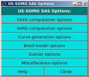
In this module you can set/change the parameters used by the SAXS/SANS (SAS) and MALS Data Processing and Simulation Module. The module has been split up into several sub-modules, as shown in the above image. The sub-menus can be accessed by clicking on their names.

In the SAXS Computation Options: section, the first entry that can be set/changed is the Water electron density (e / A^3): (default: 0.334 e/A³).
Next comes the choice between the computational methods offered: full Debye ("F-DB"), Debye with spherical harmonics ("SH-DB"), a fast methods based on FoXS (Schneidman-Duhovny et al., Nucl. Acids Res. 38, W540-W544, 2010), whose code is only available for Linux operating systems ("quick" Debye, "Q-DB"), and Crysol (Svergun et al., J. Appl. Cryst. 28, 768-773, 1995). If "Q-DB" is selected, it is possible to have at the same time the computation of the P(r) vs. r function by ticking the "P(r)" checkbox. In particular:

• F-DB. The full Debye method (Glatter and Kratky, Editors. Small-Angle X-ray Scattering. New York: Academic Press. 1982) first calculates the contrast atomic form factors for each atom i at each scattering vector q_j:

  

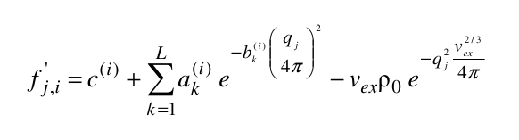
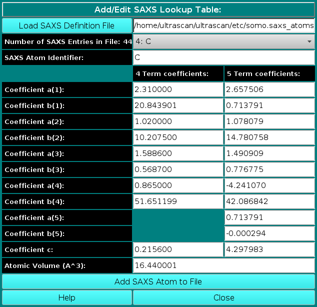
  where a_k⁽ⁱ⁾, b_k⁽ⁱ⁾, and c⁽ⁱ⁾ are the pre-exponential terms, the exponential (Gaussian) terms, and the constant term, respectively, of the atomic form factors taken from the International Tables for Crystallography and stored in the SAXS coefficients table, L is the number of Gaussian terms used (4 or 5, user-selectable in the SAS Miscellaneous Options menu, see below; for the 5 Gaussians, see Waasmaier and Kirfel, Acta Cryst. A51:416-431, 1991; Yonekura et al., IUCrJ 5:348-353, 2018), v_ex is the excluded volume of each atom retrieved from the atom definition table, and ρ₀ is the solvent electron density, stored in the US-SOMO SAXS calculation options (default: water, 0.334 e/ų). If implicit hydrogens are used, as is typical for most structures derived from X-ray crystallography studies, then structure factors derived from a Debye computation utilizing typical hydrogen positions replace the atomic form factors. The v_ex for non-H atoms stored in the somo.atom file already includes the H atoms bound to every particular group defined there (e.g., C4H3 v_ex = 31.89 Å³, C4H0 v_ex = 16.44 Å³). The I_j are then computed for each q_j as:

  

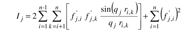
  where r_i,k is the distance between the centers of atoms i and k.

• SH-DB. The spherical harmonics method is based on a spherical Bessel function expansion of the Debye equation and is described further in (Stuhrmann, Acta Cryst. A26, 297-306, 1970; Stuhrmann et al., Proc. Natl Acad. Sci. USA 74, 2316-2320, 1977; Svergun and Stuhrmann, Acta Cryst. A47, 736-744, 1991).

• Q-DB. This is an internal implementation of the FoXS method described in Schneidman-Duhovny, Hammel and Sali, "FoXS: a web server for rapid computation and fitting of SAXS profiles", Nucl. Acids Res. 38:W540-W544, 2010. Presently, no options can be set for FoXS, which is then unable to perform parametric fitting to an experimental curve.

• P(r). A P(r) can be simultaneously computed with the quick Debye method at relatively small computational cost. Selecting this option will produce both an I(q) and a P(r) curve when running the Q-DB computation.

• Crysol. This will externally call the popular program Crysol (Svergun, Barberato, and Koch. J. Appl. Cryst. 28:768-773, 1995), whose main options can be set in the fields below. Notice: the parametric fit to an experimental curve capability of Crysol has not been implemented within US-SOMO.

Next come a series of entries where various parameters can be set:

In the Quick Debye: Bin size. Smaller bin sizes increase accuracy at the cost of increased computational time. See the FoXS paper reference for details. The default value is that used in the standard FoXS method.

In the Quick Debye: Modulation. The modulation effects the exponential decay of a point scatterer extended from the intensity at q = 0 (I(0)). See the FoXS paper reference for details. The default value is that used in the standard FoXS method.

The next three entries set some Crysol options (the first affects also the SH-DB method):

SH/Crysol: Maximun order of harmonics (default: 15). Increase this number as the size of the structure grows (max for the current Crysol implementation: 40).

Crysol: Order of the Fibonacci grid (default: 17). Increase this number as the size of the structure grows (max for the current Crysol implementation: 18)

Crysol: Contrast of the hydration shell (e/A^3): (default: 0.03 e/A³). Set this parameter to "0" if you want to run Crysol on a structure with explicit hydration waters.

Five checkboxes follow, grouped under Crysol options::

Automatically load difference intensity (default: on). After a Crysol computation, the difference intensity data will be loaded in the graphic window.

Support version 2.6 (default: on).

Support version 3.1+ (default: off).

Shell water (3.1+ only) (default: off). This is a relatively recent new Crysol feature allowing the representation of hydration waters as dummy beads placed on the bio-macromolecule's exterior surface, and their inclusion in the I(q) calculations (see Franke et al., J. Appl. Cryst. 50:1212-1225, 2017).

Crysol: Explicit hydrogens (default: off). By default, Crysol uses implicit hydrogens considered as part of the bound atom and explicit hydrogens are removed. If you wish to use explicit hydrogens specificed in your pdb, then select this option.

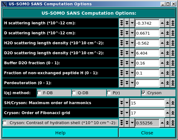
In the SANS Options: section, several parameters can be controlled:

• The hydrogen neutron scattering length can be set in the H scattering length (*10^-12 cm): field (default: -0.3742 × 10^-12 cm).

• The deuterium neutron scattering length can be set in the D scattering length (*10^-12 cm): field (default: 0.6671 × 10^-12 cm.

• The H₂O neutron scattering length density can be set in the H₂O scattering length density (*10^10 cm^-2): field (default: -0.562 × 10¹⁰ cm^-2).

• The D₂O neutron scattering length density can be set in the D₂O scattering length density (*10^10 cm^-2): field (default: 6.404 × 10¹⁰ cm^-2).

• The actual D₂O content in the sample is set in the Buffer D₂O fraction (0 - 1): field (default: 0.5).

• The fraction of non-exchanged peptide hydrogen can be controlled in the Fraction of non-exchanged peptide H (0 - 1): field (default: 0.1).

• The perdeuteration fraction can be set in the Perdeuteration (0 - 1): field (default: 0)

b(Y)_i = b(0)_i + n(H_Exch)_i * Y * [b(D) - b(H)] * [ 1- f(NH_Exch)_i]

where b(0)_i are the neutron scattering lengths of the non-H atoms at Y = 0 and n(H_Exch)_i are the number of exchangeable H attached to them (both tabulated in the hybridization table), b(D) and b(H) are the D and H scattering lengths, respectively, and f(NH_NExch)_i is the fraction of non-exchanged peptide bond H (which is 0 for all atoms except for the peptide bond N atom), all as defined in this panel (see above). The perdeuteration field is used by Cryson (see below).

As for the SAXS Computation options panel, we have listed a series of alternative methods for the computation of the SANS I(q) vs. q curves. However, only Cryson (Svergun et al., Proc. Natl. Acad. Sci. USA, 95, 2267-2272, 1998) is presently (as of June 2024) active.

The maximum number of harmonics and the order of the Fibonacci grid can be set in the corresponding fields for Cryson. Regarding the Cryson: contrast of the hydration shell field, it is automatically computed from the D₂O fraction (see Cryson manual), but the value proposed can be overridden by checking the checkbox provided and entering a different value.

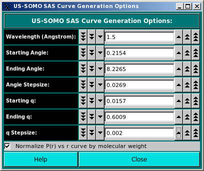
The SAS Curve Generation Options: section contains fields whose values are used in the simulation of either a SAXS or a SANS curve.
Enter either the X-ray or neutron wavelength in the Wavelength (Angstrom): field (default: 1.5 A for SAXS; for SANS, an usual value is 6 A).
The span and point density of the simulated curve can be controlled by entering appropriate values in the Starting Angle, Ending Angle, and Angle Stepsize fields, or in the corresponding Starting q, Ending q, and q Stepsize fields, where the transformation from angle units to scattering vector q units is automatically carried over by the program. Default values are 0.001 to 0.6 A^-1 q range with a 0.015 stepsize, corresponding to an angular range of 0.014 to 8.214 degrees with a 0.2 degrees stepsize for a wavelength of 1.5 A.

The Normalize P(r) vs r curve by molecular weight is selected by default. Deselecting it will cause the P(r) vs. r curves to be normalized only by their areas.

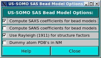
This module allows selecting the computation of the SAXS and/or SANS coefficients when generating bead models from atomic scale structures (Compute SAXS coefficients for bead models and Compute SANS coefficients for bead models checkboxes), and to optionally use the Rayleigh (Rayleigh, Proc. Royal Soc. London A84:25-46, 1911) structure factors for spheres of uniform electron density (Use Rayleigh (1911) for structure factors checkbox). This procedure is still under development, and will be fully described elsewhere.

The Dummy atom PDB's in NM checkbox is used when uploading bead models whose scale units are not in Å but in nm, like some DAMMIN/DAMMIF-generated models.

In the SAS Guinier Options menu, the options controlling the Guinier analysis of SAS data can be set, and the various operational modes can be then launched. After setting/revising the options and the parameters, three different Guinier analyses can be launched by pressing "Process Guinier" (conventional Guinier, ln[I(q)] vs. q²), "Process CS Guinier" (cross-section Guinier for rod-like particles, ln[q I(q)] vs. q²), or "Process TV Guinier" (transverse Guinier for disk-like particles, ln[q² I(q)] vs. q²), respectively.

The general Guinier options that can be set/modified are:

• Guinier: Maximum q * Rg: value (default: 1.3), where "Rg" is the overall z-average square radius of gyration <R_g²>_z.

• CS Guinier: Maximum q * Rc: value (default: 1), where "Rc" is the cross-section z-average square radius of gyration <R_c²>_z for rod-like macromolecules.
• TV Guinier: Maximum q * Rt: value (default: 1), where "Rt" is the transverse z-average square radius of gyration <R_t²>_z for disc-like macromolecules.

The specific Guinier, CS Guinier and TV-Guinier options that can be set/modified are:

• The Minimum q value for Guinier search (default: 1 × 10^-7 Å^-1).

• The Maximum q value for Guinier search (default: 0.5 Å^-1).

• The Minimum q^2 value for Guinier search (default: 1 × 10^-14 Å^-2).

• The Maximum q^2 value for Guinier search (default: 0.25 Å^-2).

  Note that by changing a value in the q fields, the corresponding value in the q² fields is automatically updated, and vice-versa.

• The Limit maximum q to maximum q*Rg, q*Rc or q*Rt (not active in Search mode) checkbox: if selected, in manual mode the linear regression will first operate within the q/q² ranges selected above, and then check sequentially every q value starting from the maximum value to see if the resulting R_g, R_c or R_t obeys the q*Rg, q*Rc or q*Rt Guinier approximation validity limits set in the appropriate fields (see above). If not, the data point corresponding to that q value is removed, and the regression repeated until a q_max value is found at which the q*Rg, q*Rc or q*Rt Guinier approximation validity limits are respected.

• Use SD for fitting. When checked, a weighted linear regression is performed, using the data associated SDs as weights.

• Repeat the analysis after discarding points over the regression line by more than SD of (value). When selected, outliers laying by more than the entered SD value from the linear regression fit can be automatically discarded from the fitting, and the regression performed again until no more outliers are found. This is particularly useful when one or a few "bad" data points are in the middle of the examined q or q² range (default: 2 SD).

• Save Guinier results to csv file (filename). Guinier analysis results can be saved in a csv-style file by selecting this checkbox. The saved file will contain, in separate lines if more than one dataset is processed: source file, a note reporting if the analysis was successfully performed ("OK" or "Failed"), either the <R_g²>_z or the <R_c²>_z or the <R_t²>_z value (depending on which type of Guinier was chosen), its associated fitting SD, the corresponding root mean-square value [<R_g²>_z]^1/2 or [<R_c²>_z]^1/2 or [<R_t²>_z]^1/2, its associated SD, the <I(0)>_w value, its associated SD, either the derived <M>_w or <M/L>_w/z or <M/A>_w/z value (depending on which type of Guinier was chosen), its associated SD, the Δe(p-s), the q_min value, the q_max value, the q_min*R_x value, q_max*R_x value (with x = g, c or t), the starting point used in the linear regression, the ending point used in the linear regression, the number of points used, a list of rejected points (if any), the χ² of the regression, the sample concentration (mg/ml) associated with the data, the partial specific volume (cm³/g) associated with the data, the I(0)(std) experimental value of the standard used for normalization, the slope of the linear regression, its associated SD, and if the SD weighting was used. At the end of the header line of the file, it is also reported which kind of fitting range was used (manual or search).

• Save processed q, I(q) data to csv file. Processed I*(q) data (see below) can be saved in another csv-formatted file by selecting this checkbox.

• Search for best Guinier range. By selecting this option, the program will optimize the q² range for best linearity, but still within the chosen q² limits. the "Use SD for fitting" option is allowed in this mode, but not both the "Limit maximum q to maximum q*Rg, q*Rc or q*Rt" or the "Repeat the analysis after discarding points over the regression line by more than SD of" options.

• The Minimum number of points: to be included in the analysis (default: 10).

• The Maximum number of points: to be included in the analysis (default: 100).

The MW and M/L computation options section deals with the parameters that are necessary to perform a correct calculation of <M>_w or <M/L>_w/z or <M/A>_w/z.

Note: from the July 2024 release, the calculations necessary to put the experimental data on an absolute scale can be done directly in the HPLC/KIN module, generating what we have called "I#(q)" and "I*(q)" datasets/files. These files will be automatically recognized and no further calculations will be performed on them, except using an entered concentration for the "I#(q)" datasets.

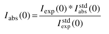
Otherwise, the conversion from the corresponding experimental <I_exp(0)>_w value is done by first putting the data on an absolute scale by normalizing for the intensity extrapolated to 0 scattering angle of a known standard, , according to:

Then the reduced in g mol^-1 are obtained as:

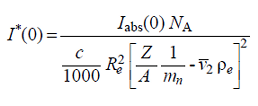
where N_A is Avogadro's number, c is the sample concentration [mg ml^-1], R_e is the diffusion length of the electron [cm], m_n is the nucleon mass [g] (note: from 2019, this value by default is taken as 1/N_A), is the partial specific volume of the particle [cm³ g^-1], ρ_e is the solvent electron density [e/cm³], and Z and A are the number of electrons and of nucleons, respectively, in the particle, whose ratio is usually taken as a constant specific for each class of biomacromolecules.

If a series of I(q) SAXS curves have been uploaded in the SAS module (for instance, from the HPLC/KIN module), it is possible to set/modify their associated parameters by pressing the Set Curve Concentration, PSV, I0 standard experimental button (see here). As stated above, for already fully pre-processed I*(q) datasets, proper values for these parameters were already employed, and will just be shown by accessing this module. The same partially holds for I#(q) datasets, for which a c value can instead be entered.

When no parameters are entered via the Set Curve Concentration, PSV, I0 standard experimental module, the program will utilize the values as set in this section of the Guinier Options module, which also contains the other parameters necessary for the computation of the <M>_w or <M/L>_w/z or <M/A>_w/z values. In particular:

• A value for the concentration can be entered in the Default concentration (mg/ml) field. (Default: 1 mg/ml).

• A value for the partial specific volume can be entered in the Default partial specific volume (ml/g) field. (Default: 0.72 ml/g).

• The Default diffusion length (cm) is set here. (Default: 2.82 × 10^-13 cm).

• The default Electron/nucleon ratio Z/A is set here. (Default: 1.87; average value for proteins).

• The default Nucleon mass (g) is set here. (Default: 1.6606 × 10^-24 g).

• By selecting the Use I0 standards for normalization checkbox, the experimental value and its theoretical value under the same experimental (T, pressure) conditions will be used to normalize the SAXS data.

• The Default I0 standard experimental (a.u.) will be used if a is not associated with the data, or entered via the Set Curve Concentration, PSV, I0 standard experimental module. (Default: 0.01633 a.u.; this value is set equal to the default value for water at 20 °C, the standard used in US-SOMO, see below).

• The I0 standard theoretical (cm^-1) refers to the absolute for the chosen standard. The default value (0.01633 cm^-1) is that for H₂O at 20 °C.

After properly setting all options/parameters, the computations of the three different Guinier data analysis processes can be launched by pressing either the Process Guinier, or the Process CS Guinier, or the Process TV Guinier buttons.

In the SAS Miscellaneous Options menu, several controls and limits can be set.

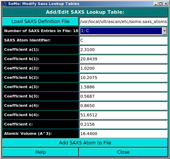
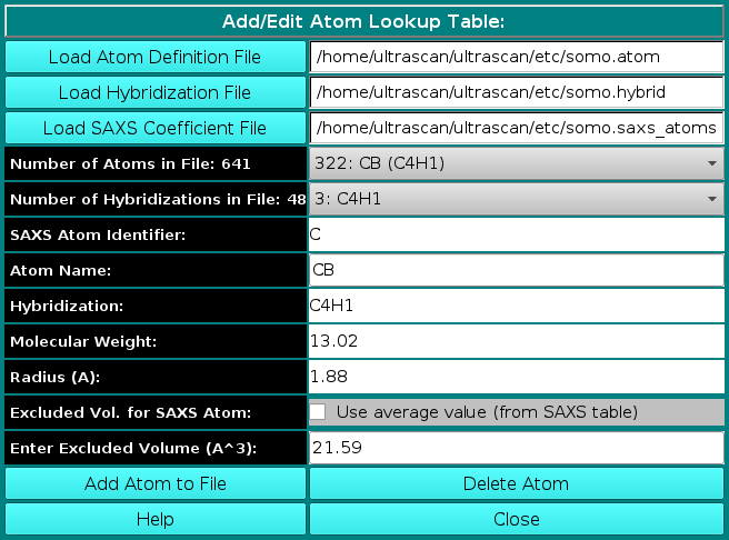
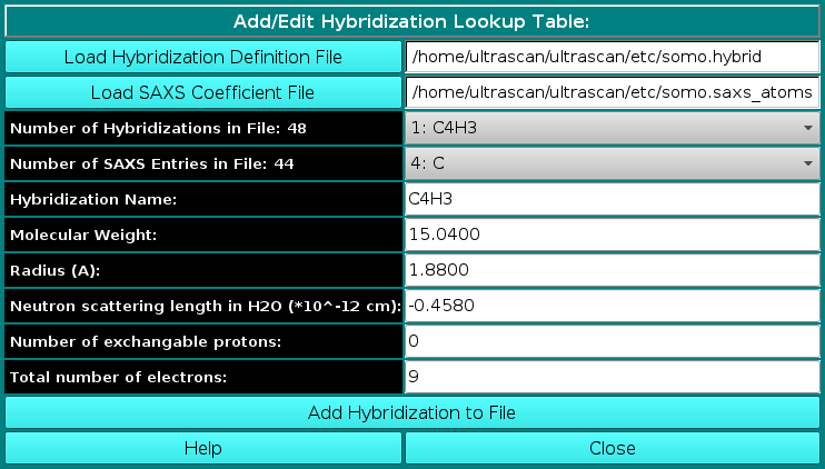
In order to properly compute the I(q) vs. q and P(r) vs. r curves, the SAS module utilizes the atom definition (default: somo.atom), hybridization (default: somo.hybrid) and SAXS coefficients (default: somo.saxs_atoms) tables.
Different tables can be selected by pressing the Load Atom Definition File, Load Hybridization File, and Load SAXS Coefficients File buttons. See the main help for further explanations on the content and use of these tables.

Next come a series of checkboxes:

• Use 5 term Gaussians for native SAXS computations. This option relates to the approximation used to compute atomic scattering factors in Debye calculation of SAXS curves (see SAXS Computations Options above). See the Add/Edit SAXS Lookup Table for more explanations on this subject. By default, this checkbox is On, but since 5 term Gaussians are not available for all entries in the somo.saxs_atoms table, in case this happens for one or more particular atom(s) in the PDB file under examination, 4 term Gaussians will automatically be instead used for that/those particular atom(s).

• Always ask 1/angstrom or 1/nm. By default, the SAS module operations assume that the length units are Angstrom. By selecting this box, a pop-up window will appear everytime a curve is uploaded/calculated, asking to define the length units (default: Off).

• Calc I(q) ask for grid. Selecting this checkbox will disable the pop-up window asking to use an already uploaded curve to set the grid for I(q) vs. q computations (default: On).

• I(q) curves in 1/Angstrom and I(q) curves in 1/nanometers. These mutually exclusive checkboxes define the length units when computing the I(q) vs. q curves (default: 1/Å).

• Expt. data in variance. This will set if the errors reported in the experimental data files are SD or variances (default: SD).

• Disable I(q) scaling. Selecting this checkbox will disable the scaling function at the end of an I(q) vs. q computation (default: Off).

• Kratky fit. The default method will perform fitting of I(q) vs. q data, but Kratky fitting (q²*I(q) vs. q) can be selected by ticking this checkbox. (Default: Off).

The Excluded volume scaling field allows to modify by a % value the excluded volumes of the non-water atomic groups as tabulated in the atom definition table.

Pressing the Clear remembered molecular weights button will erase stored MW from the program's memory.

A different q range can be entered in the I(q) curve q range for scaling, NNLS and best fit (Angstrom) two fields.

Two new checkboxes where added starting from the March 2023 release:

• List zero contribution entries in NNLS fits. When dealing with large datasets to be NNLS-fit to a target, it is not practical to list all individual datasets in the progress window. Therefore, the default mode involves now listing only the contributing datasets. The full listing can be restored by checking this checkbox (default: unselected).

• Truncate P(r) fits to Dmax of target. When dealing with NNLS fits of P(r) datasets generated from flexible structures, the D_max calculated from the experimental curve is an average over the multiple conformations present in solution. Each individual model-derived P(r) instead has a D_max than can potentially exceed the experimentally-determined value. Selecting this checkbox will truncate any calculated P(r) curve to the experimentally-determined D_max value (default: unselected).

This document is part of the UltraScan Software Documentation distribution.
Copyright © notice.

The latest version of this document can always be found at:

http://somo.aucsolutions.com

Last modified on June 25, 2024.