Manual

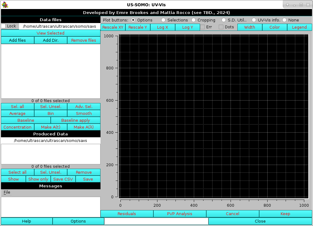This module is made available from the July 2024 release, and was developed for the analysis of time-and wavelength-resolved absorbance data collected with either a Diode Array Detector (DAD) or a Charged-Coupled Device (CCD). These data are originally produced as a matrix-format array containing in columns the absorbance values as a function of time for each wavelength covered by the detector, and in lines their values as a function of wavelength. The UV-Vis module will first generate individual Absorption vs. time (A(t) vs. t) files for each wavelength present, which can be subsequently transposed into Absorption vs. wavelength (A(λ) vs. λ, where λ is the greek symbol for wavelength) for each available time point.

At the top of the left-side panel, you can pre-select a directory where your data are stored. Clicking on this field (shown in the picture above is the /home/ultrascan/ultrascan/somo/saxs path) will open a directory navigator where you can selected another directory. Checking the Lock checkbox will make the selected directory the default one upon re-starting the application.

In the bottom command bar, some important options can be set, as described here, by pressing the Options button. It is advisable to check them before proceeding with data processing.

To begin with data processing, in the current set-up you first have to load a file where the wavelengths covered by your DAD or CCD are listed. The current format for this file is a single column listing all the wavelengths sequentially (separated by character return).
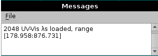
Use the Add files button to navigate the directory tree until you find the wavelengths-containing file. Upon loading, in the progress window at the bottom left side of this module a message will be printed listing the number of wavelengths and the [starting:ending] wavelengths:

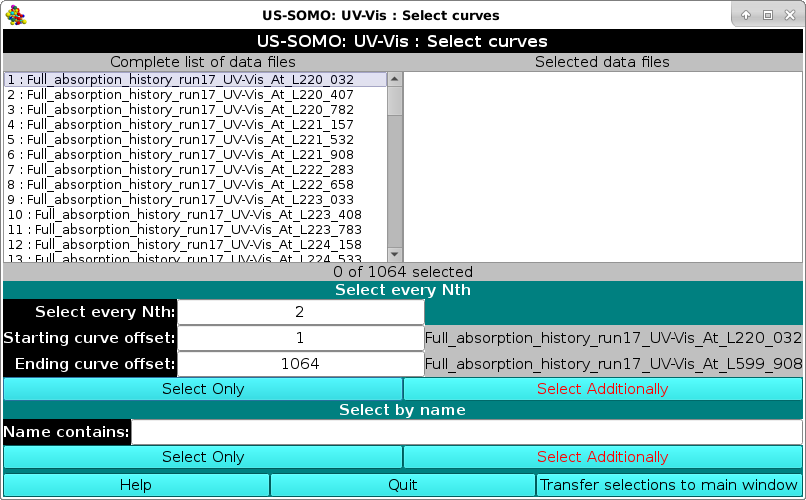
You can now load your array containing the Absorption vs. time data for each wavelength, by using again the Add files button to navigate the directory tree (note: you can also use the Add Dir. to directly select a directory, but you must be sure that it contains only the single file with your array). Upon choosing a file, to avoid potential mismatches a message will pop-up alerting the user of the already loaded wavelengths:

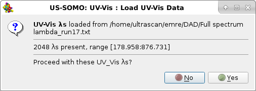Pressing Yes will allow the program to proceed. To avoid loading data collected for wavelengths that will not be utilized in the subsequent analyses, another pop-up window will present the option of subselecting a range of wavelengths for loading the corresponding Absorption vs. time data:

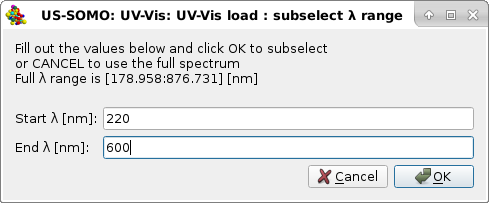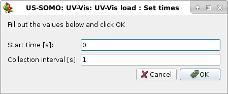
In this example, we restrict the data to the to the 220-600 nm wavelength interval, and we will proceed by pressing Ok. Pressing Cancel will instead load the data for the full wavelength range. A final pop-up window will then let you define the starting time (0 in this example) and the collection interval (1 s in this example) for the data that, we remind, are stored in a file as an array containing the Absorption values at each wavelength in lines, and their time-evolution in columns (a column containing the times is not present in this format):

Pressing Ok will finally launch the data loading, populating the upper left-hand window with the data labels (format "originalfilename_UV-Vis_At_Lxxx_xxx", where "L" stands for "lambda" and "xxx_xxx" is the wavelength at which that particular Absorption vs. time data sequence was recorded. At the same time, the Progress bar in the bottom row will signal the advancement of data loading:

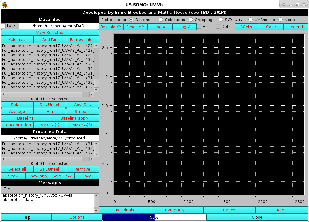Note that since individual files are created from the loaded array containing the Absorption vs. time data for each wavelength, the Produced data section is also being populated with the same filenames. The completion of the loading process is then signaled in the progress window at the bottom left:

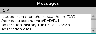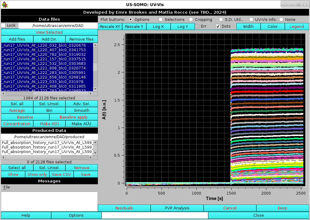
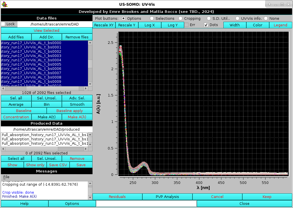
Pressing Select all will show the entire loaded dataset in the graphics window:

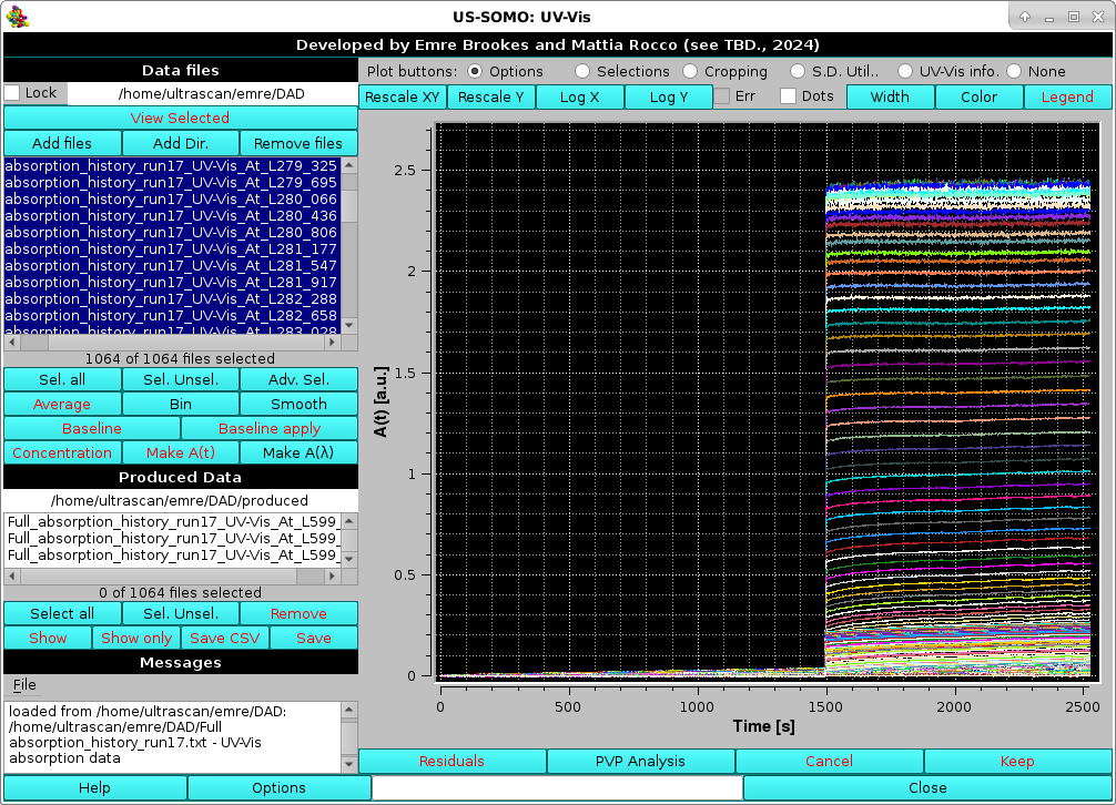In this case, we are dealing with a baseline region followed by the injection of a sample. The graphic window now has the correct labels for the x (Time [s]) and y (A(t) [a.u.] axes. The list of the loaded data can be scrolled using the right-hand bar, and for long data filenames (such as in this case) the full wavelength values, which are positioned at the end of the filename, can be revealed by scrolling with the bottom bar, as done in the picture above.
Pressing again Select all will unselect all selected data.
The content of each file can be visualized in a text format by pressing View Selected (no editing is allowed). Note that if multiple files are selected, each one will be opened in a separate viewer; however, View Selected becomes unavailable if ten or more files are selected.
Since upon loading the initial array has been subdivided into single Absorption vs. time data for each wavelength files, on pressing Remove files a pop-up panel will be shown asking what action should be taken:

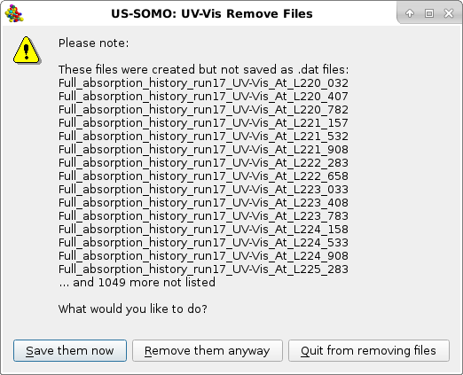Save them now will open up the directories navigator for saving the newly created individual files, Remove them anyway will clear all the selected files, Quit from removing files will abort this operation.
Individual files can be selected and visualized by clicking on them in the file list, holding "Shift" while clicking on separate files will select and visualize also all files in between the selected ones, holding "Ctrl" while clicking on separate files will select and visualize just those files, as shown in the example below:

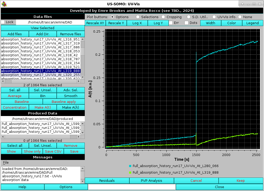For the image above, the Legend button in the top row above the graph has also been pressed, resulting in the two selected files filenames being shown below the graph.
As with all the US-SOMO graphics windows, graph regions can be zoomed-in with the mouse (holding the left mouse button), and zoomed-back in steps by clicking on the mouse right button. Pressing the Rescale XY or Rescale Y buttons in the top bar above the graph will also provide other means of rescaling.
Log X and Log Y will change the respective axes to log₁₀ scales, and the buttons will then be re-labeled Lin X and Lin Y, respectively; pressing them again will then revert the respective axes to linear scaling.
The default data visualization mode is by lines connecting the data points. It can be changed to individual points (squares) mode by checking the Dots checkbox; the Err checkbox will show the points as empty diamonds with their associated y-axis standard deviations, if present, as vertical bars. Width will lead to a stepwise increase of the width of either lines or symbols for four cycles, reverting then to the original width. Color will sequentially change the color of each shown data set each time it is pressed.

All the above functions belong to the Options set as selected by the round checkbox of the Plot buttons row positioned above the buttons bar.
Checking the Selections checkbox will change the buttons bar to four new buttons:

Select visible will become active (the red color on the labels signals no availability at the moment) once a part of the graph has been selected (zoomed) with the mouse. It is a practical way of selecting just one of a few of the dataset shown in the graph, and will affect the selected files listed in the top left panel.
Likewise, Remove visible will become active once a part of the graph has been selected (zoomed) with the mouse. pressing it will lead to the same pop-up panel as described above if the selected data have NOT yet been saved.
For both those buttons, cliking on the mouse righ button thus reverting to the full graph will make them inactive.
Save plots will open up the directories browser where a location and a filename can be chosen to save all the data currently shown in the graphics window as a csv-formatted file.

Checking the Cropping checkbox will change the buttons bar to seven new buttons:

As for the Selections, the Cropping buttons become all available when a part of the graph is selected using the mouse/left button, (only Crop Zeros and Crop Common are available when files are just displayed after selection).

Crop Common will crop all selected files so that they have identical x-axis values by dropping points outside of the union of all selected file's x-axis values.
Crop Vis(ible) will remove what is shown in the graphics window. For instance, this is practical way to trim the data on the x-axis.
Crop to Vis(ible) will select only what is shown in the graphics window after zooming with the mouse.
Crop Zeros will remove data having zero or negative values in the intensity columns (discouraged: a warning panel will pop-up, asking the user whether she/he really wants to proceed, since experimental zero or negative values can have statistical significance).
Crop Left and Crop Right will remove one point on the left or right of the selected data, respectively.
Undo will undo the last cropping action performed.

Checking the S.D. Util. checkbox will change the buttons bar to two new buttons:

This utility was devised to better evaluate the associated SD in SEC-SAXS chromatograms (see here). As most DAD or CCD-generated data do not carry any SD information, it could be useful to define them by analyzing flat regions of time-dependent absorbance and evaluating the oscillations in their values. By pressing the SD eval. button, two vertical red lines will be superimposed on the initial region of the chromatogram, and two red-background fields controlling their position will appear in the bottom row of the commands below the graphics window:

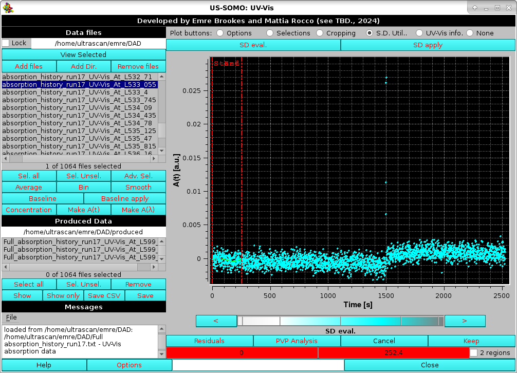An additional checkbox, 2 regions, if selected will duplicate the vertical lines and their associate fields (colored magenta this time), allowing to utilize more than one flat region for the SD estimation (not shown).

The SD evaluation is carried out by fitting the data included between each zone with a 3^rd degree polynomial, and taking the RMSD of the fit as the SD. If two regions are chosen, the final SD will be an average between the values computed from each region.

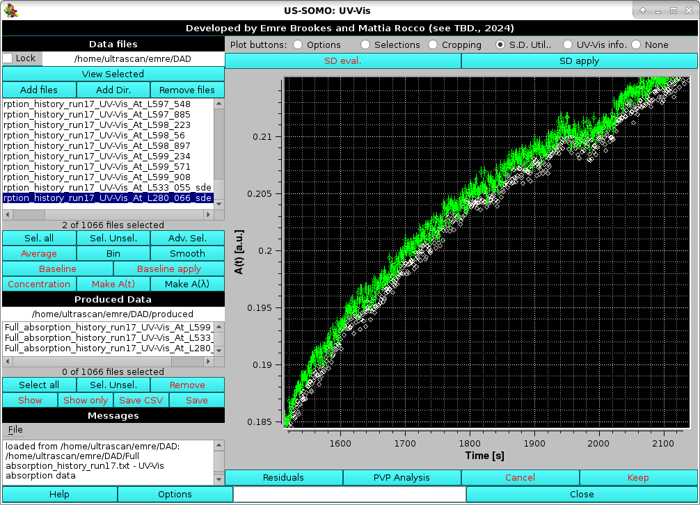
After adjusting the zone(s) for the SD evaluation, pressing Keep will accept the values, and the SD apply button becomes available. Pressing it will apply the SD calculation to any selected A(t) dataset, generating files with the extension "_sde".

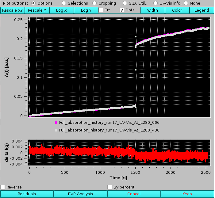
In this example, the SD were evaluated in a baseline region at a wavelength where no changes were recorded in the experiment's time frame, and then applied to the A(t) data at λ=280.066 nm. In the image below, these A(t) data with SD (green) are compared with the ones without SD (white) at the very close λ=280.436 nm in a restricted time interval:

Checking the UV-Vis info checkbox will list first the source of the wavelengths for the current dataset, then their number and range, followed by the chosen wavelength with its associated extinction coefficient:

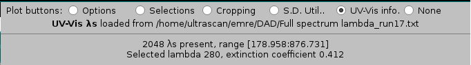Finally, checking the None checkbox will make all the buttons disappear.

At the bottom of the graphics window there are four buttons:

Residuals will become active when two files have been selected, and pressing it will compare them showing their differences in an additional graph below the main one:

checking Reverse will reverse the order of the comparison, while checking By percent will show their % difference instead of the absolute values (not shown). Pressing again Residuals will exit from this function.

PVP Analysis is not (yet) available for the current (July 2024) US-SOMO release.

Cancel and Keep are buttons that become available when other functions are enabled (see below).

Returning to the commands on the left-side, below the list of loaded data files, the Adv. Sel. button will open up a module where advanced selection options are available:

The user can consult the Help present for the same functions in the HPLC/KIN module of US-SOMO, see here.

The Average button is not available for A(t) vs. t) data, its use will be described when dealing with A(λ) vs. λ data (see below).

Bin can be used to reduce the number of time points in A(t) vs. t files. On pressing it, a pop-up panel will ask the number of points to be used for binning:

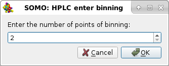After choosing a suitable bin size, on pressing Ok a new series of the selected files will be produced with extension "-bin#", with "#" being the number of points chosen. The newly-generated files will be automatically selected and shown in the graphics window. Cancel will abort the operation.

Smooth can be used to treat particularly noisy data. On pressing it, a pop-up panel will ask the number of points to be used for smoothing:

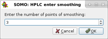After choosing a suitable number of points over which the smoothing is to be applied, on pressing Ok a new series of the selected files will be produced with extension "-sm#", with "#" being the number of points chosen. The newly-generated files will be automatically selected and shown in the graphics window. Cancel will abort the operation.

Baseline is a function that is used to define a region of a single A(t) vs. t file to be averaged and subsequently subtracted to the entire file. Pressing it will add some functions at the bottom of the graphics window:

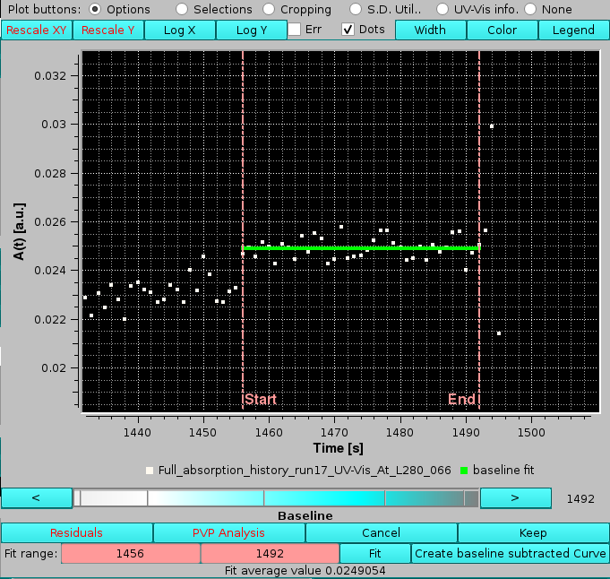After zooming in a candidate region, two vertical pink bars can be moved either by entering times in the pink-colored Fit range: boxes, or by acting with the mouse on the white-to-cyan-scale bar-wheel below the graph (the Legend has been enabled for this image) after having clicked on one of the pink boxes, or by clicking on the the "<" and ">" buttons placed at its sides. The green solid line will appear automatically on setting the limits, showing the current average between the points in the selected interval, whose value is also reported at the bottom. The Fit button can be used if the green line does not appear automatically.
The Create baseline subtracted Curve button can be used to generate the baseline-subtracted curve for the current file (not shown in the graphics window, only appended to the files list in the left-hand side panel; the filename will the the same with appended "_blc#_#######", with "#_#######" being the subtracted baseline average value).
Pressing Cancel will exit from the Baseline function without retaining the chosen baseline region.
Pressing Keep will instead save the chosen baseline region limits, which can then be used to generate baseline-subtracted curves for any other loaded data files.
The effect on subtracting a baseline can be seen in the image below, where the evident drifting of the A(t) vs. t values at the selected wavelength have been offset, allowing a correct determination of the absorbance of the sample at the time of sample injection:

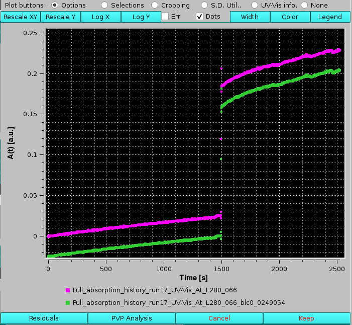If a baseline has been defined on a file, and kept, the Baseline apply button can be used to generate baseline-subtracted curves, Any number of files can be simultaneuosly selected and then baseline-corrected. The module will evaluate the average baseline value for each file using the common baseline region as defined in the original file. The newly generated, baseline subtracted curves (with their names appended as explained above) will be then automatically shown in the graphics window:

The Concentration and Make A(t) buttons are available only when A(λ) vs. λ data are selected (see below).

The Make A(λ) button is used to transpose A(t) vs. t data into A(λ) vs. λ data. At least two A(t) vs. t files must be selected before this button becomes available.
To demonstrate its usage, we will first crop the above-generated baseline-subtracted data, to remove the zone before sample injection. The first operation is to select with the mouse a large part of the no-sample region:

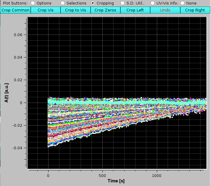Pressing Crop Vis will make a pop-up panel appear:

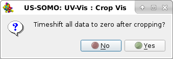This function will allow to optionally reset the time axis to 0 after cropping, so that t=0 coincides with the sample injection. Press No to decline. If Yes is pressed, another pop-up panel will appear stating the details of the timeshift operation following cropping:

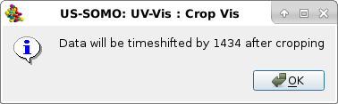Press Ok to continue.
This operation can be repeated with a finer zooming, until the exact sample injection point is left as the data time origin:

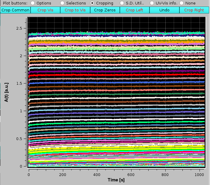We can now proceed with Make A(λ). At the end of the operation, the new files generated will have the extension "AL_t_####", where "####" reports the progressive time (note: in this particular case, since the data were baseline-subctrated, the extension is "AL_t_bs####"), and the A(λ) vs. λ data are automatically shown in the graphics window:

The dangers of not carefully evaluating the zone for baseline correction can be seen by comparing the A(λ) vs. λ at the same t=8 s without (lime green) and with (pink) baseline correction:

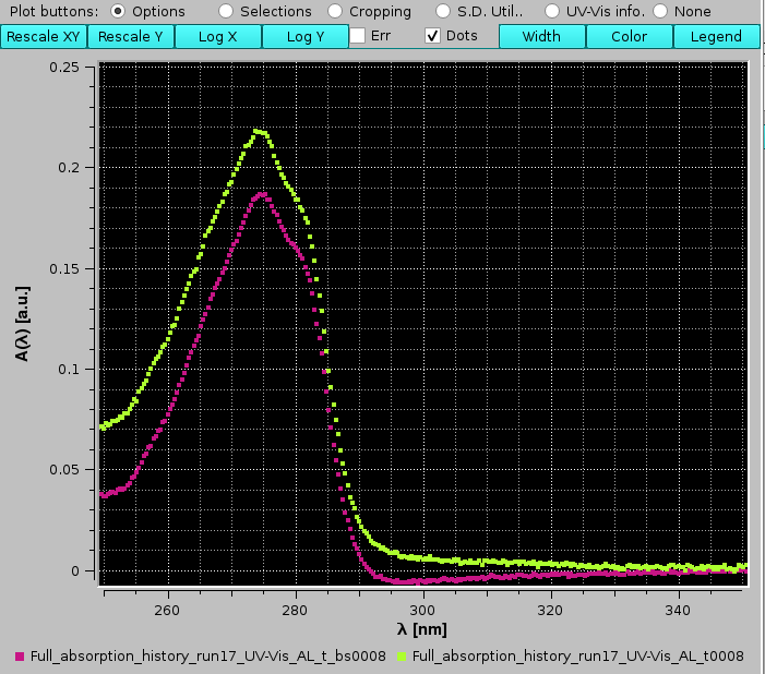where an overcorrection in the 290-330 nm range can be seen for the baseline subtracted spectrum.

If two or more A(λ) vs. λ are selected, the Average button becomes available. Pressing it will produce a pointwise (for each λ value) average A(λ) vs. λ file, containing also the SD of the mean, with extension "f#_firstt_lastt", where "#" is the number of files averaged, and "firstt","lastt" are the times associated with the first and the last averaged files.

Given the very fine λ intervals usually provided by DAD or CCD detectors, Bin can also be utilized for A(λ) vs. λ files to reduce the number of independent λs. See above for the Bin usage.

Concentration, available when only a single A(λ) vs. λ file is selected, will open below the graphics window an advanced module for spectral analysis, including full scattering correction and concentration determination:

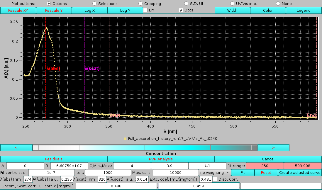The first thing one notices is that the λ chosen for the concentration determination, the "standard" 280 nm at which extinction coefficients are calculated, indicated with the vertical red line labeled "λ(abs)" in the graph, is not centered on the absorbance maximum. The extinction coefficient for this sample was therefore recalculated at the λ maximum, 274 nm, and found to be 0.481 mL mg^-1 cm^-1. These values were then entered in the λ(abs) [nm] and Extc. coeff. [mL/(mg*cm)] fields, respectively. In addition, a λ at which a simple scattering correction is evaluated, 320 nm, is entered in the λ(scat) [nm] field. We can now see the vertical red line correctly positioned at the top of the absorbance peak, and a new vertical magenta line labeled "λ(scat)" positioned at λ=320 nm:

The A(λ,abs) [a.u.] and A(λ,scat) [a.u.] fields show the respective values as linearly interpolated from the absorbances read from the data at the closest wavelengths to those selected in the λ(abs) [nm] and λ(scat) [nm] fields.
The bottom line reports the concentration (c, [mg/mL]) calculated according to three different ways:

• Uncorr.: the "raw" calculation, just dividing the absorbance measured at the peak λ (A(λ,abs) [a.u.]) by the extinction coefficient;

• Scat. corr.: the absorbance at the scattering λ (A(λ,scat) [a.u.]) is subtracted to the absorbance measured at the peak λ A(λ,abs) [a.u.] before dividing by the extinction coefficient;

• Full corr.: in this procedure, described below, a full scattering curve is evaluated in an interval where no absorption is taking place, by fitting the absorbance data to the theoretical power law, Abs(λ)=A+B*(λ)^-C, with A, B, and C the coefficients. The power law is then used to calculate a full scattering curve covering the entire wavelength range of the data, which is then pointwise subtracted to the original curve. The concentration is then calculated dividing the absorbance at the peak wavelength of the corrected spectrum by the extinction coefficient. However, since the refractive index of the solution and the differential increment of the solute refractive index dn/dc both change as a function of the wavelength, affecting the scattering by the solute, a dispersion correction option has also been implemented (Disp. Corr. checkbox; see below).

In the Fit controls: line, we have first the fitter ε: value (default: 1e^-7), then the number of iterations allowed Iter: (default: 1000), and finally the maximum number of calls Max calls: (default: 10000). Next comes a pulldown box where a fit weighting method can be chosen:

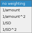Since DAD- or CCD-produced data usually do not carry associated SD values, the default method is no weighting. The options are listed in the image above. For instance, SD weighting can be used if the analyzed spectrum was produced within this module as an average of a number of spectra each without associated errors, resulting in the SD of the average having been calculated.

Pressing Fit will launch it, with these results:

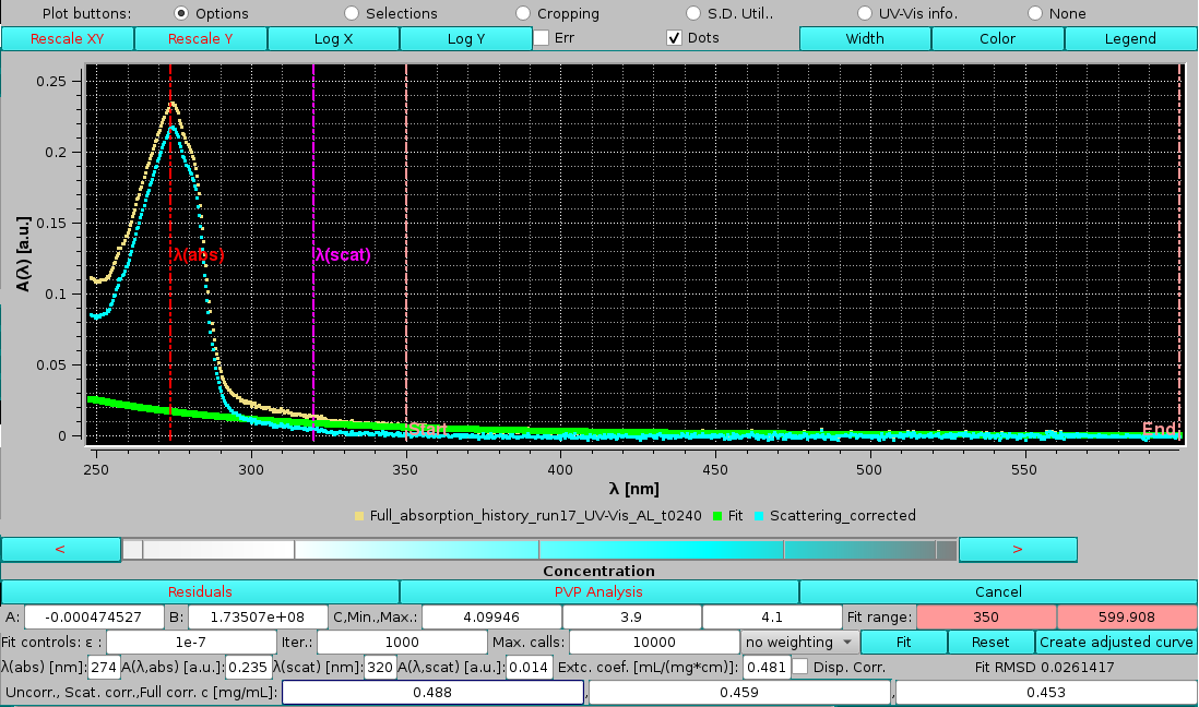In this example, the C term was found to be almost equal to the upper limit, and the offset A term almost negligeable. The resulting scattering curve is shown in green, and the scattering-corrected spectrum in cyan. The third box on the last line, reporting the concentration after full scattering correction, is now populated. Note how this value, 0.453 mg/mL, is very close to the one calculated using just the absorbance value at λ=320 nm for the scattering correction, 0.459 mg/mL, consistent with a small scattering contribution for this sample, which nevertheless affects significantly the calculated concentration, as indicated by their difference from the uncorrected value, 0.488 mg/mL.

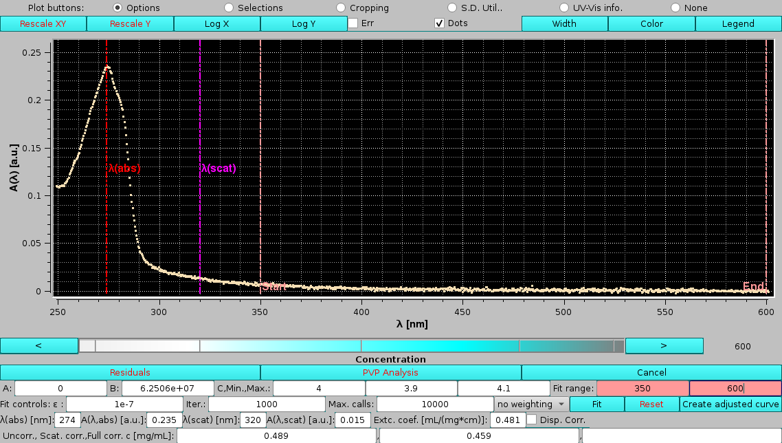
We can now assess the effects of changing the limits for the scattering power fit. After manually inserting values of λ=330 nm and λ=550 nm as the lower and upper limits, respectively, the Reset button is pressed to re-initialize the fit parameters. Pressing Fit will then produce these results:

with a slightly improved RMSD and a slightly lower offset value, while the exponent is practically the same. The fully corrected concentration is also slightly lower than the one calculated with the previous λ limits.

The effect of using the dispersion correction (Disp. corr. checkbox selected) can be now evaluated using the other previous settings:

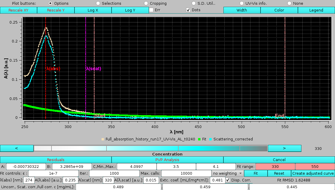with very similar results, suggesting that the dipersion correction plays a minor role when the scattering contribution is not high. Note that we had to initialize the fitting with a lower limit on the C term, although its final value is again close to the upper limit. The RMSD is noticeably worse in this case. Note also that the wavelengths shown in the graph are not the ones calculated with the dispersion correction (see below) and used for the fit, but the original ones.

The dispersion correction is based on recalculating the effective wavelength in solution based of optical constant K in the Rayleigh-Gans-Debye scattering theory:

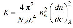
where n_λ and (dn/dc)_λ are the λ-dependent refractive index of the solution and differential increment of the refractive index of the solute as a function of the concentration. We can rewrite:

leading to:

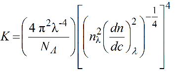
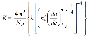
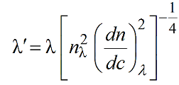
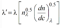
These λ-dependencies can be derived by fitting with power laws the square roots of n_λ and (dn/dc)_λ values calculated as a function of λ using, for example, the program SEDNTERP3 (downloadable here). Remember to properly set also the temperature at which these calculations are made! Therefore, in the US-SOMO UV-Vis Options entries are provided to store these values calculated for the current solvent and sample.

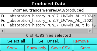To begin with, in the first field the path to a default directory that is automatically created inside the directory from where you first loaded data is shown (in this example, /home/ultrascan/emre/DAD/produced). Clicking on this field will open up the directories navigator where you can create a specific new directory that will be then used as a new location where to save the data.

Below the directory field there is the list of produced files, which can be selected by clicking on them (with the usual rules for Shift and Ctrl), and that can be managed using the provided buttons:

• Select all will select all data listed in this section.

• Sel. Unsel. will select only previously unselected data listed in this section.

• Remove will delete all data selected in this section. As usual, a pop-up warning panel will alert the user before proceeding.

• Show will additionally show in the graphics window the data selected in this section.

• Show only will show in the graphics window only the data selected in this section.

• Save CSV will save in a single csv-style file the data selected in this section.

• Save will save in individual .dat files the data selected in this section.

This document is part of the UltraScan Software Documentation distribution.
Copyright © notice.

The latest version of this document can always be found at:

http://somo.aucsolutions.com

Last modified on June 24, 2024