Manual

Last updated: June 2024

The Integral Baseline method is based upon the assumption that capillary fouling deposits are formed in proportion to the sample concentration while exposed to the beam, and that neither the buffer nor the instrumental background are contributing to this effect. That deposition on the capillary does occur is clearly proven by the fact that a steady SAXS signal is maintained even after completion of the protein elution. The theory underlying the Integral Baseline correction procedure can be found here.

To help the user decide if a baseline correction is needed, and to find a proper region of SAXS steady state signal at the end of the chromatograms, the currently implemented Integral Baseline method requires an analysis on blank frames. These "Blanks" (no less than 10 frames, possibly at least 20 or more must be available) should have been collected well before the void volume, and should preferentially be the same ones that were then averaged and subtracted from all the data collected during the chromatogram development.

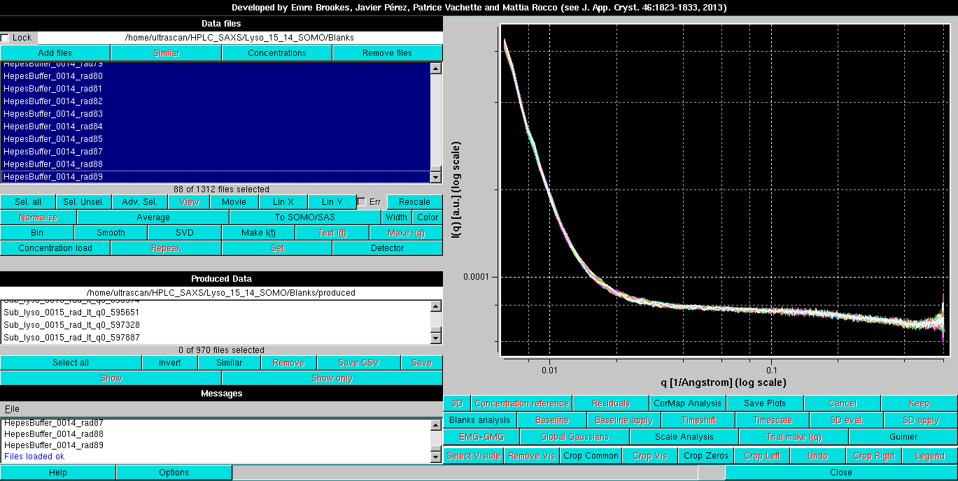
After Blanks files have been loaded using the Add files button (see above), their analysis is launched by pressing the Blanks analysis button. The module will automatically convert the I(q) vs. q frames into I(t) vs. t chromatograms:

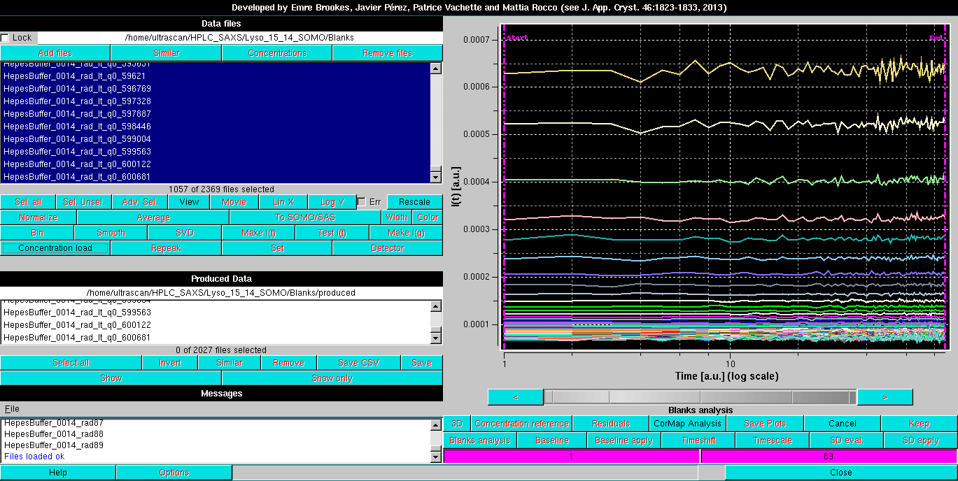
The two vertical magenta lines and their corresponding fields at the bottom of the buttons' zone define the beginning and end regions for the Blanks analysis. By clicking on one of the fields and then moving the mouse on the grey-scale bar-wheel just below the graphics window, these limits can be changed. This can also be done in steps of a single frame by clicking on the "<" and ">" buttons placed at the extremities of the bar-wheel. Alternatively, the limits can be manually changed by entering a numerical value in their respective fields.

The Blanks analysis is performed by clicking on the CorMap Analysis button. This will launch a pairwise Correlation Map analysis (see here for a descrption of the CorMap implementation in the US-SOMO HPLC/KIN module). Before the analysis is effectively launched, a pop-up panel will appear:

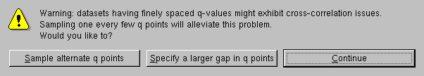
It was found during the implementation of the Blanks analysis that finely spaced q values might result in cross-correlation effects in the CorMap analysis (see also here). Therefore, this pop-up panel will allow to chose a sampling in q space to eliminate or at least alleviate this problem. Since usually a one-every-two values sampling is sufficent, this can be directly done by pressing the Sample alternate q points button. Larger sampling intervals can be chosen by entering an integer value after pressing the Specify a larger gap in q points button. If no sampling is wanted, the Continue button should be pressed.
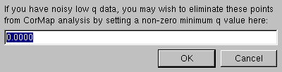
A second pop-up option will also allow to start the CorMap analysis above a chosen q_min value, to avoid including very noisy, low-q values in the analysis:

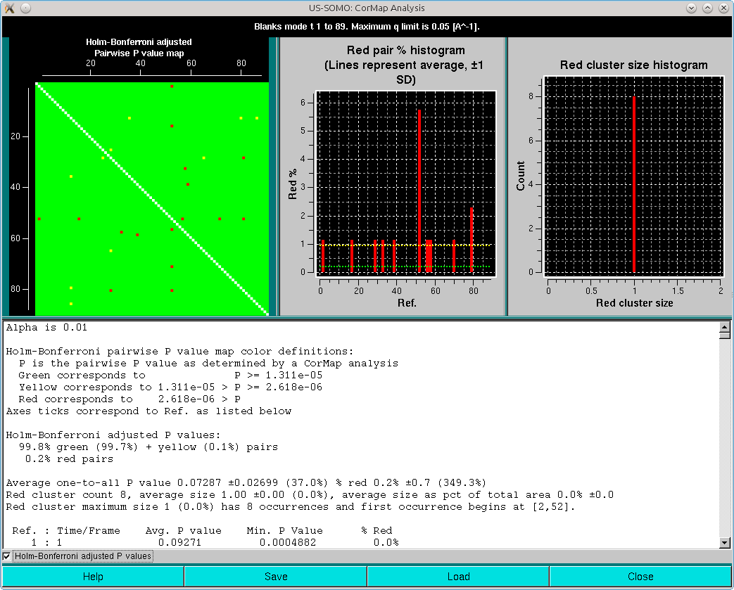
After these choices are made, the analysis is effectively launched, and the results are shown in a new pop-up panel (see here for a full description of the CorMap implementation):

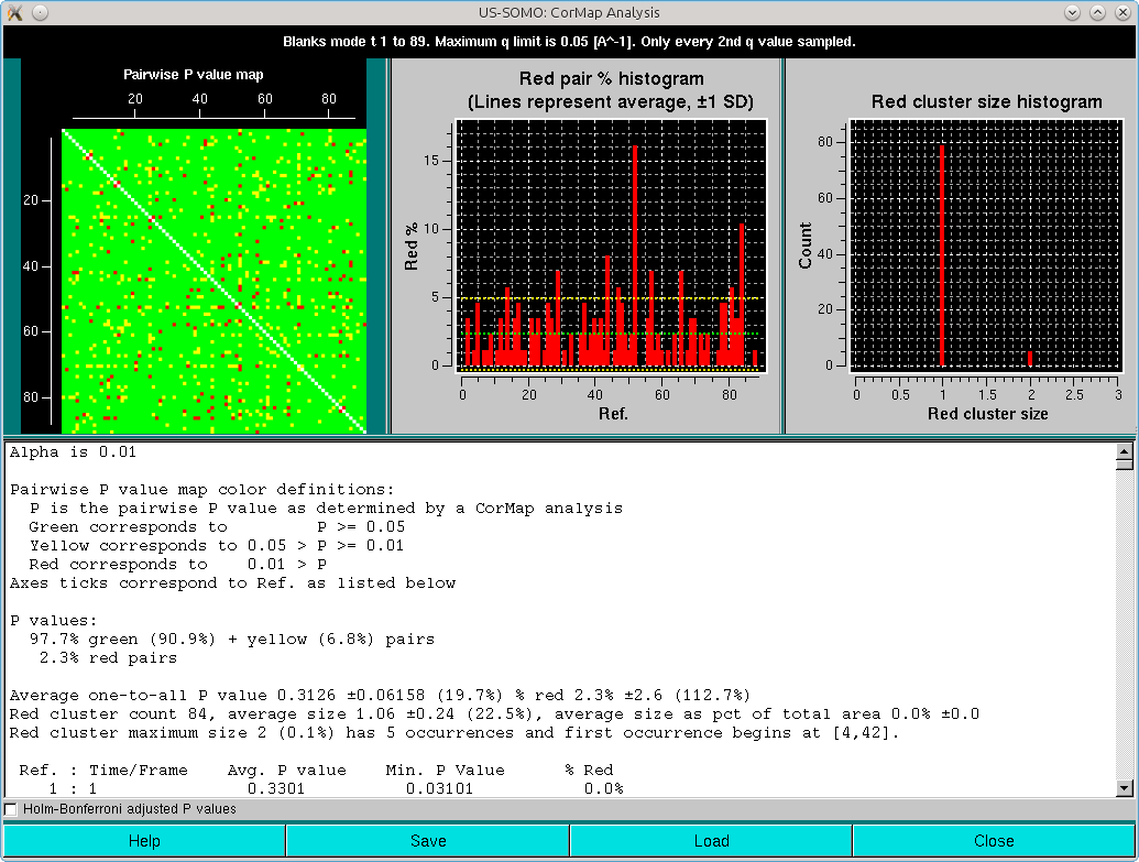
The pop-up panel begings by reporting on the top bar the type of analysis (here "Blanks mode t 1 - 89"), the max q limit used (here 0.05 Å^-1), and the sampling used (here "Only every 2^nd q value selected").

Three plots are present on the top of the panel:

• A Pairwise P-value map, a square matrix in which the square (i,j) contains the P-value resulting from the (i,j) curves represented by a three color code: green for P ≥ 0.05, yellow for 0.01 ≤ P ≤ 0.05, and red for P < 0.01. The labels on the axes correspond to the reference numbers given to the analyzed frames (see below).

• A Red pair % histogram plot as a function of the time/frame number, derived from the analysis of the pairwise P-value map in terms of the distribution of values between the three classes with an emphasis on the % of red squares.

• A Red cluster size histogram, derived from an evaluation of the average size of clusters of horizontally and/or vertically adjacent "red" squares. After careful examination of several indicators derived from the P-value map analysis, this was chosen as the most reliable to determine the global similarity between all frames of the considered subset.

• A summary of the resulting P values pairs in terms of the green+yellow sum % and red % values.

• The average one-to-all P value ± its SD (in parentheses the % SD value) and the % of red values ± their SD (in parentheses the % SD value.)

• The red cluster count, their average size ± their SD (in parentheses the % SD value) and their average ± SD size as % of the total area.

• The red cluster maximum size (with its % in respect to the total area), the number of occurences of that cluster size, and the position of the first occurence.

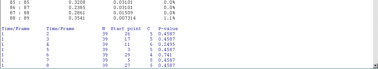
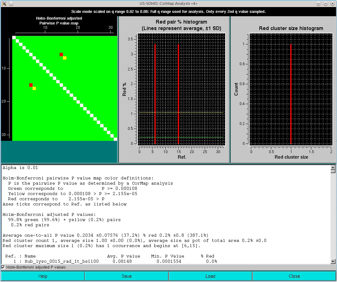
At the end of the text area, a checkbox is present. If selected, the paiwise analyses will be adjusted for multiple testing using the Holm-Bonferroni approach (Holm, S. A simple sequentially rejective multiple test procedure. Scandinavian Journal of Statistics 6:65-70, 1979; see here):

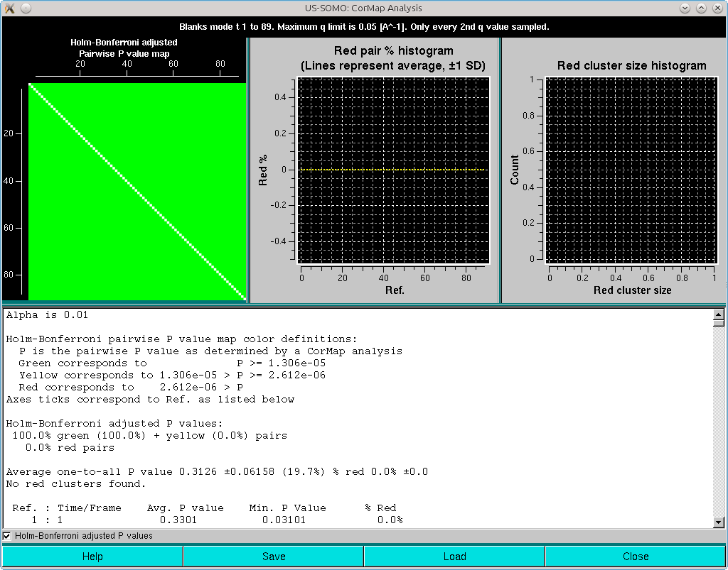
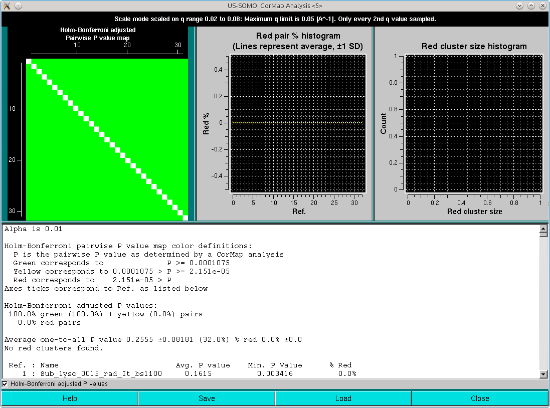
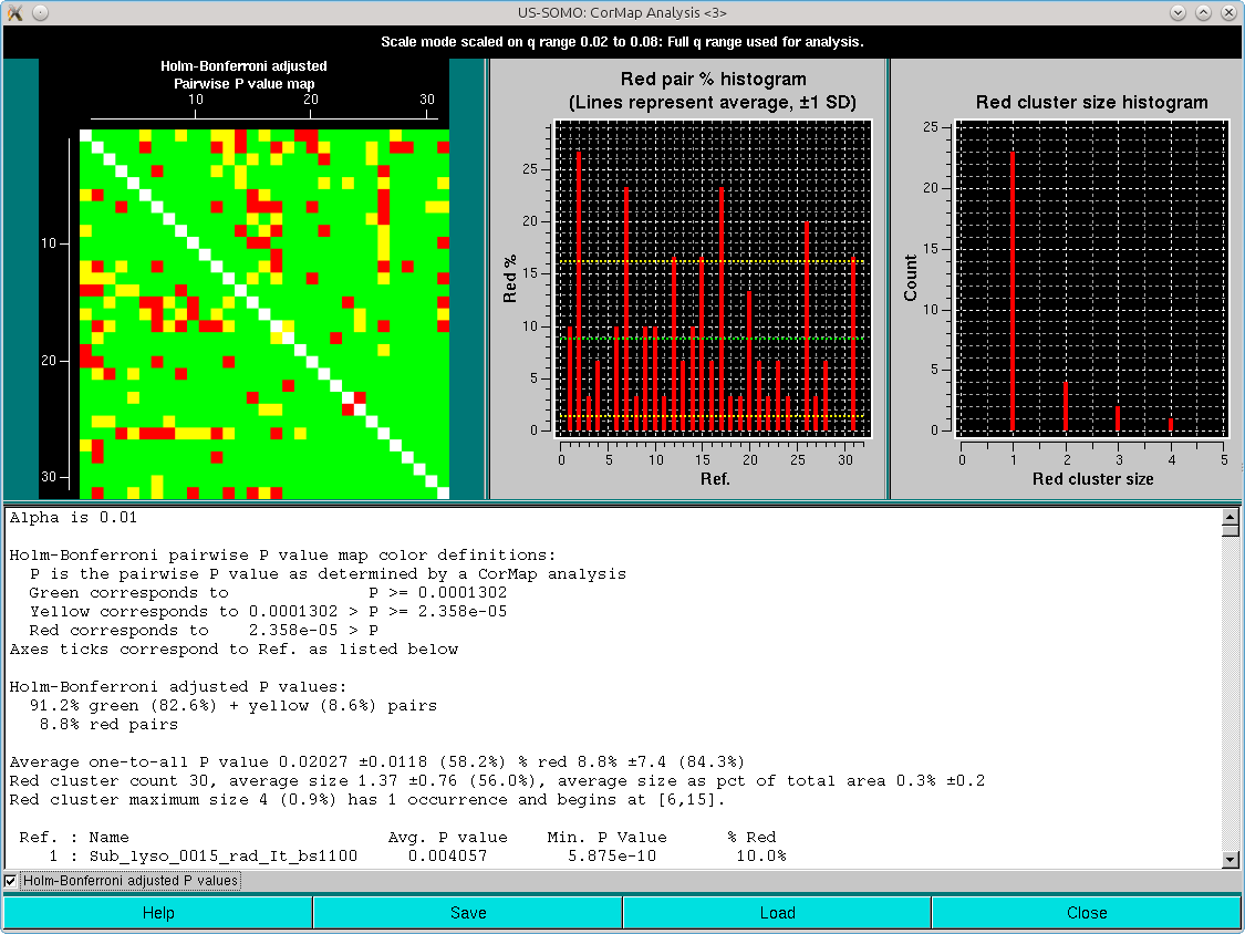
Note that in this case the Holm-Bonferroni multiple testing adjustment on a dataset where a one-every-two q-values sampling was applied has produced a completely green pairwise P-values map. Without sampling, this is what is obtained without the Holm-Bonferroni adjustment:

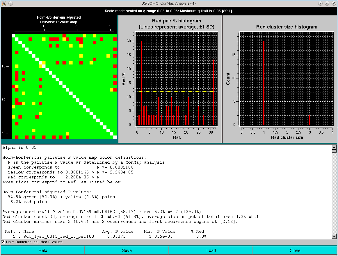
and with Holm-Bonferroni adjustment:

All data listed in the CorMap analyis pop-up window can be saved in a csv-type file with the Save button. Previously analyzed datasets can be recalled with the Load button.

After closing the CorMap analysis window, the Blanks data can be accepted by pressing the Keep button. Cancel will instead discard the current CorMap analysis.

The Integral Baseline analysis of the actual sample frames can then begin. Contrary to what was required in our previously developed Integral Baseline method, the current version requires that all I(t) vs. t chromatograms must be selected before hitting the Baseline button.
In any case, on pressing Baseline a first pop-up warning message will always appear:

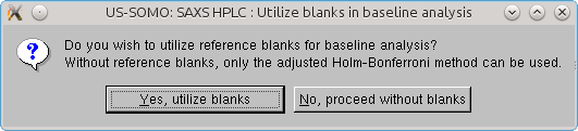
This allows the user to proceed without using a Blanks reference set to judge if a stable baseline has been reached at the end of the chromatograms. In this case, only the Holm-Bonferroni adjusted pairwise comparison will be used.

If Blanks are to be used, a second pop-up warning message will appear:

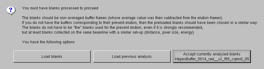
alerting that a blanks analysis is needed to proceed any further, and offering up to three options:

• Load blanks, which will allow to load I(q) vs. q Blanks files to be subjected to the analysis as described above;

• Load previous analysis, which will allow to select a previously saved Blanks analysis cvs file;

• Accept currently analyzed blanks (followed by the filename of the currently analyzed blanks).

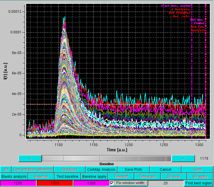
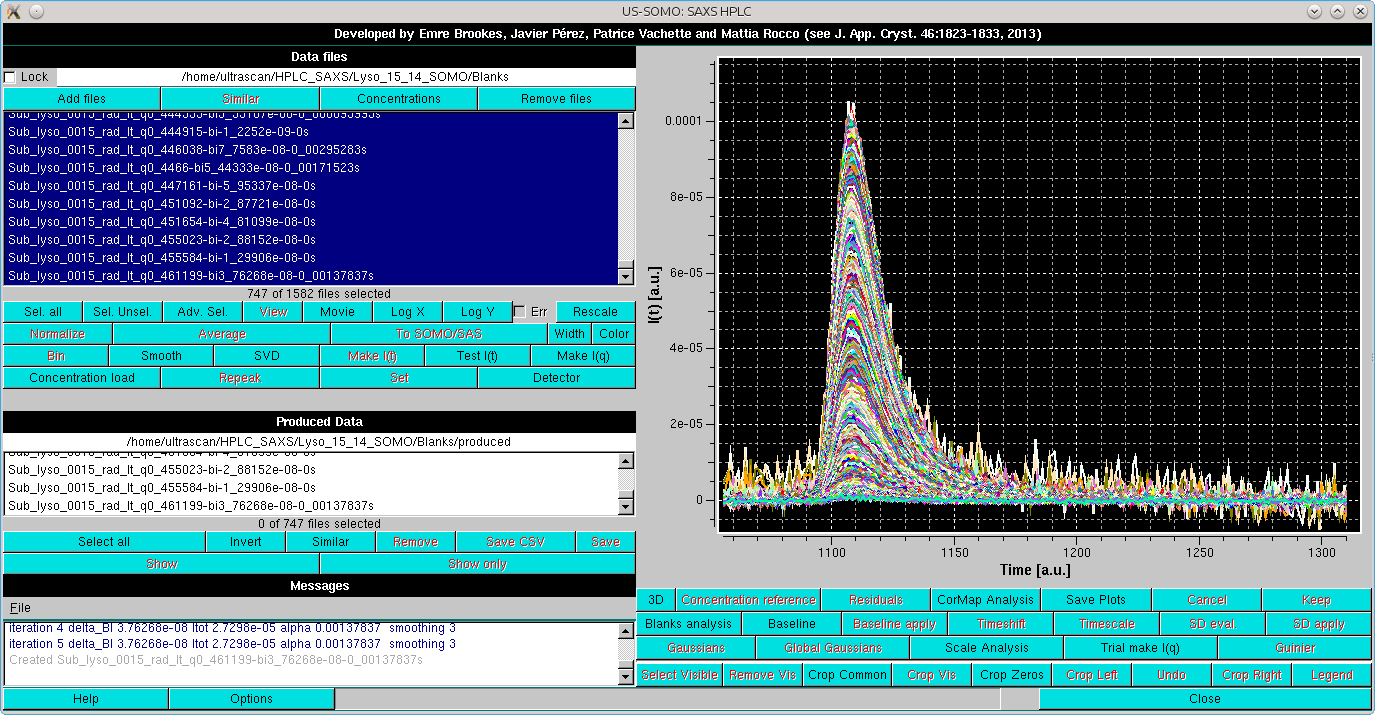
After pressing OK, the graphics window will present all the selected I(t) vs. t chromatograms and switch to the Baseline mode of analysis:

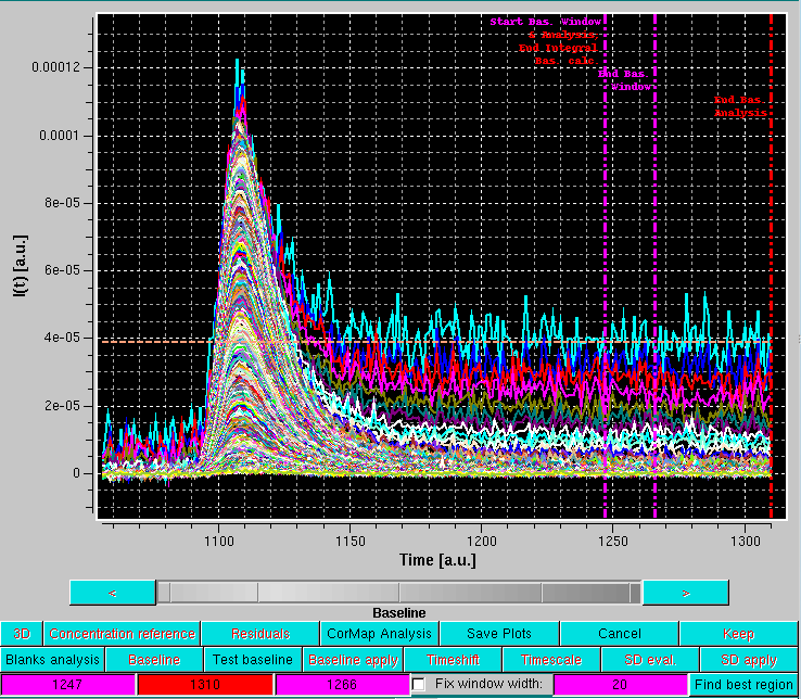
As shown in the image above, this superimposes to the selected chromatograms three vertical lines on the right side, the last two lines of buttons under the graphics window are replaced by three colored fields (magenta-red-magenta), and a dashed line is drawn horizontally (orange). In addition, a Fix window width checkbox with its associated magenta-colored field in now present (default: 20 frames, unchecked), as well as a new Find best region button.
The first vertical magenta line, which by default is positioned at 75% of the available frames, has multiple usages:

• It defines the starting frame of a sliding window over which a CorMap analysis will be carried out;

• It will also define the first frame where the CorMap analysis will start;

• When the Integral Baseline is calculated, it will be the end point of the computations (but the calculated baseline, which will be constant beyond this point, will be then subtracted up to the last frame).

The vertical red line defines the end for the sliding window analysis (default position: 5 frames from the end of the available frames).

The horizontal orange line represents the average intensity across the current window of the lowest q-value among the selected I(t) vs. t chromatograms.

It is important to remind that the baseline is set to be at zero at the beginning of the data on the left side.

The positions of the three vertical lines are indicated in the three background color-coded fields. By cliking on one of the fields, the corresponding vertical line position can be changed using either the grey-shades bar-wheel, or the "<" and ">" buttons at its sides. Manual values can be also entered.

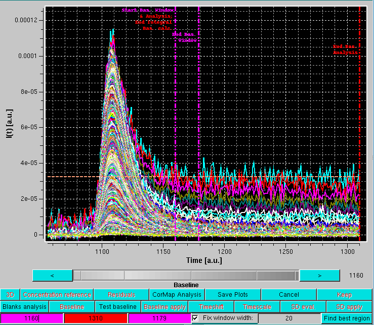
If the Fix window width checkbox is not selected, moving either of the two vertical magenta lines will also change the width of the sliding window.

It is then best to first define a window width by moving either one of the vertical magenta lines, and then fix it by selecting the Fix window width checkbox. At this point, the entire window can by positioned by using either of the two vertical magenta lines. It is suggested to position it in a region where there is still some visible intensity decay, as shown below:

The baseline analysis is then completed by pressing the Find best region button.

This will launch a special CorMap analysis in which first a global CorMap calculation will be carried out between the entire range of frames from the first vertical magenta line to the vertical red line. Subsets of this CorMap analysis corresponding to the sliding window regions will then be extracted and compared with the average of all possible CorMap analysis results extracted from the pre-analyzed Blanks data for a sliding window of the same size.

In addition, the analysis will calculate the integrated average intensity at each frame of all the I(q) values from the minimum q-value selected up to the q_max defined in the Options panel (default: 0.05 Å^-1).

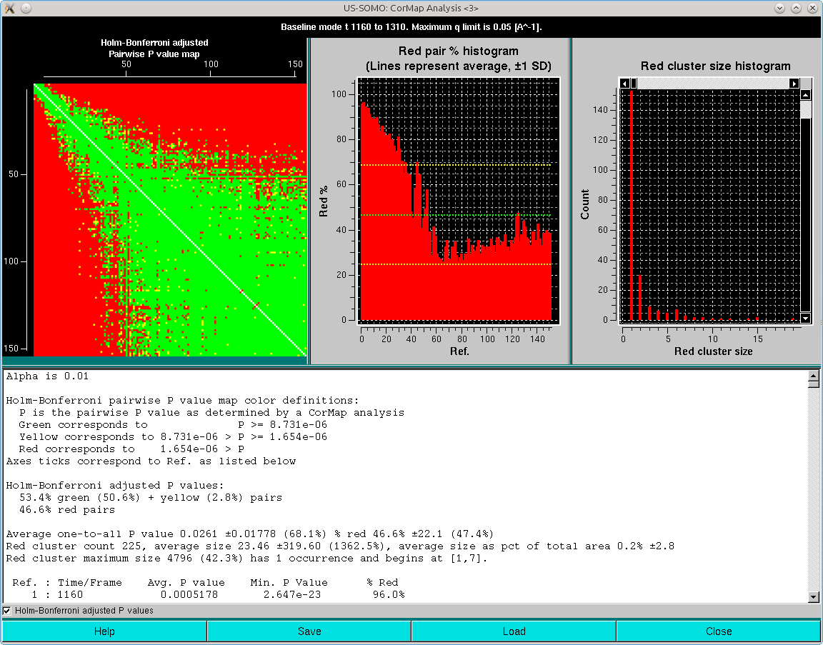
The results will appear in two pop-up panels. The first one is analogous to the one appearing after the Blanks analysis:

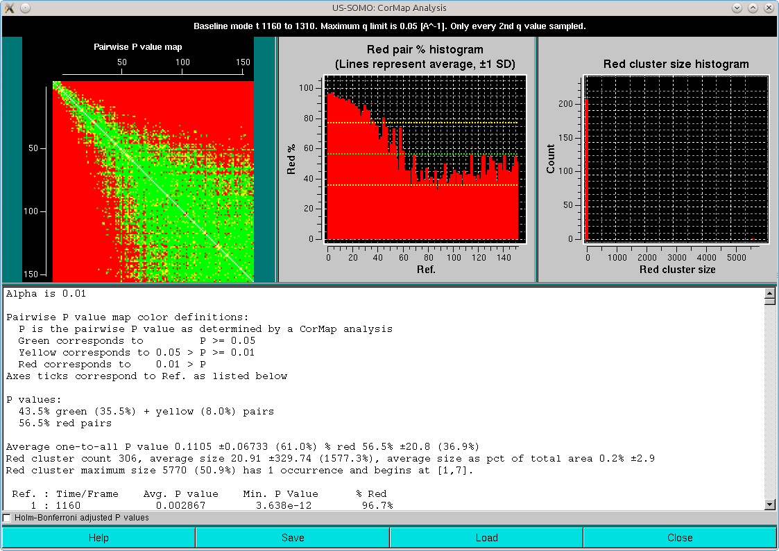
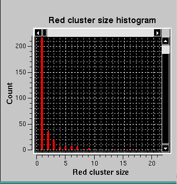
Here, it can be appreciated the almost completely red left and top sides of the Pairwise P value map plot, originating from the fact that regions on the descending side of the elution peak were included in the analysis. This also heavily affects the right-side Red cluster size histogram, with an almost invisible huge size (≈5000) but extremely low count cluster greatly compressing the scale. If we zoom on the low red cluster size region, this is what becomes visible:

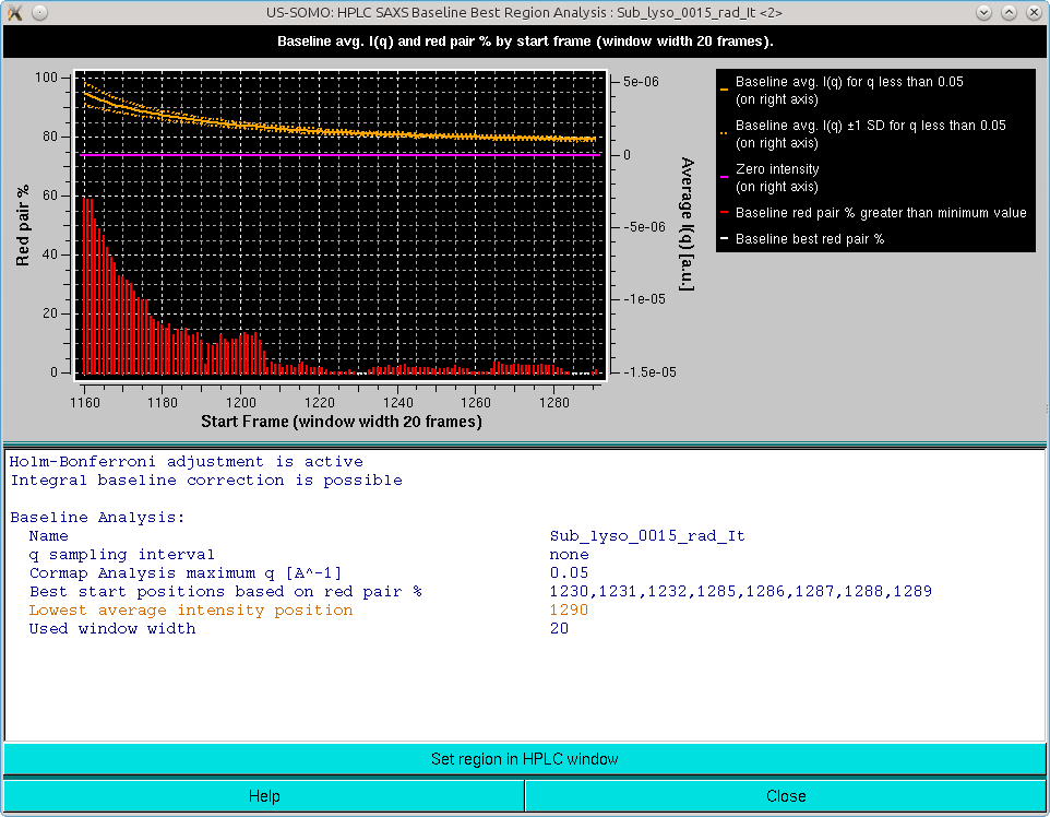
But most relevant is the second pop-up panel that will appear on top of the first:

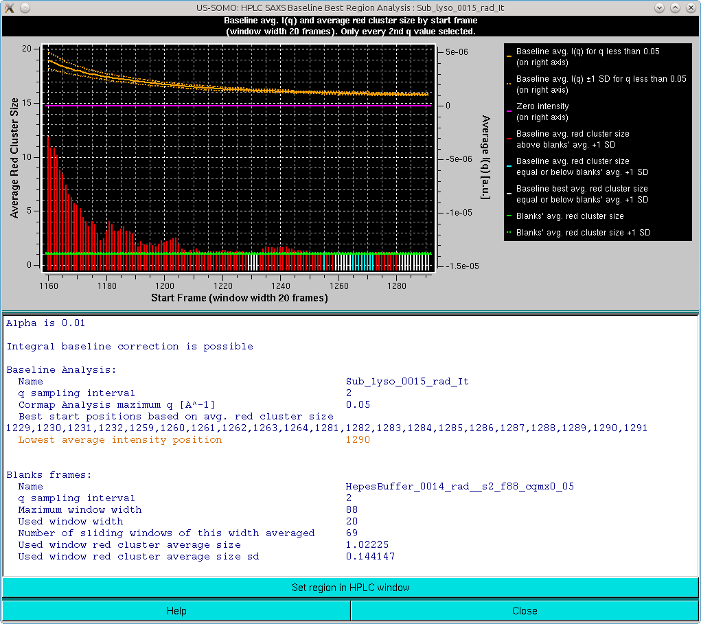
The graph in this panel is composed of two plots, both as a function of the starting window position. The bottom histogram (left-side y-axis scale) reports the average red cluster size for each window in the sliding window ensemble. The horizontal green solid line defines the Blanks average red cluster size for all possible windows of the same size as the sliding window utilized for the Sample analysis (the dotted line represents + 1 SD). The bars in the histograms are colored red when they are above the Blanks + 1 SD value, while cyan and white when they are ≤ the Blanks + 1 SD value, with the white being the lowest value(s) (equal values are possible).

The top plot (right-side y-axis scale) reports the averaged I(q) for q ≤ the q_max value (0.05 Å^-1 by default, as set in the Options), as the solid orange line, with the dotted orange lines representing ±1 SD. The solid magenta line defines the zero value expected for blanks-subtracted data when only buffer is present.

The goal of this combined analysis is twofold:

• To find region(s) of steady-state intensity;

• To compare the average integrated I(q) intensity with the zero value expected for pure buffer conditions.

• If the average integrated I(q) ±1 SD vs. starting frame position plot is always above the zero reference line and there is at least one occurrence of an average red cluster size being equal or less than the Blanks' average red cluster size +1 SD, the message "Integral baseline correction is possible" appears.

• If the average integrated I(q) ±1 SD vs. starting frame position plot is always above the zero reference line but the average red cluster sizes are always higher than the Blanks' average red cluster size +1 SD, the message "Integral baseline correction would be possible, but no steady-state end region has been identified" appears.

• If the average integrated I(q) ±1 SD vs. starting frame position plot crosses and goes below the zero reference line, irrespective of the average red cluster size status, the message "Integral baseline correction is not recommended" appears.

• The root name of the files analyzed;
  
• The q sampling interval;
  
• The CorMap analysis q_max;
  
• A list of the best starting positions for end frames (that span a length equal to the chosen sliding window size) where the average red cluster size is within 1 SD similar to those of the Blanks (white bars in the histogram; if no white bars are present, green bars will be listed; if neither white of green bars are present, a single, lowest count bar will be listed, colored yellow in the histogram);
  
• In orange color, the frame position of the lowest average integrated intensity.

• The root name of the Blanks frames files utilized in this analysis;
  
• Their q sampling interval;
  
• The maximum available sliding window width;
  
• The used sliding window width;
  
• The number of sliding windows averaged;
  
• The red cluster average size for the used sliding window;
  
• And its associated SD.

If the averaged integrated intensity -1 SD reaches at some point the zero line, then no Baseline correction is likely necessary.

If the averaged integrated intensity -1 SD at some point crosses and goes +1 SD below the zero line, then other issues might be present, such as incorrect Blanks subtraction, or drifting problems. In the latter case, a Linear Baseline correction might be indicated (see here).

If the averaged integrated intensity is always above +1 SD of the zero line, then an Integral Baseline correction could be necessary. The second condition warranting it is that there is an end region where a sufficient number of Sample frames (equal to the sliding window size by definition) is judged by the average red cluster size of the Pairwise P value Map to be similar within +1 SD of the average Blanks frames. Those are the starting frames listed in the first block of summary information, but beware of the presence of a single yellow-colored starting frame: it means that no frames passed the stringent Pairwise P value Map average red cluster size test, and that the listed frame is only the one having the lowest average red cluster size (which can be much higher than the Blanks average red cluster size). The user could try repeating the analysis using a different (smaller) sliding window size. Check also the starting/ending positions to be sure to include an appropriate end region for this analysis.

When both the Integral Baseline applicability conditions are met, the user could automatically transfer the position of the window into the Baseline module, by clicking on the Set region in the HPLC window bar at the bottom of the an analysis window. This will open a pop-up panel:

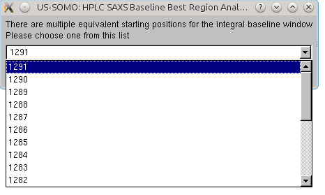
listing all possible starting positions for the baseline window, beginning with the farthest one. The user should pick a position matching with the lowest average integrated intensity frame position (orange colored text). If more than a lowest average integrated intensity frame is available, it is advisable to pick an earlier one, to avoid a potential undercorrection when integral baseline subtraction is performed. Once a position is chosen, clicking on OK will transfer it to the Baseline module panel:

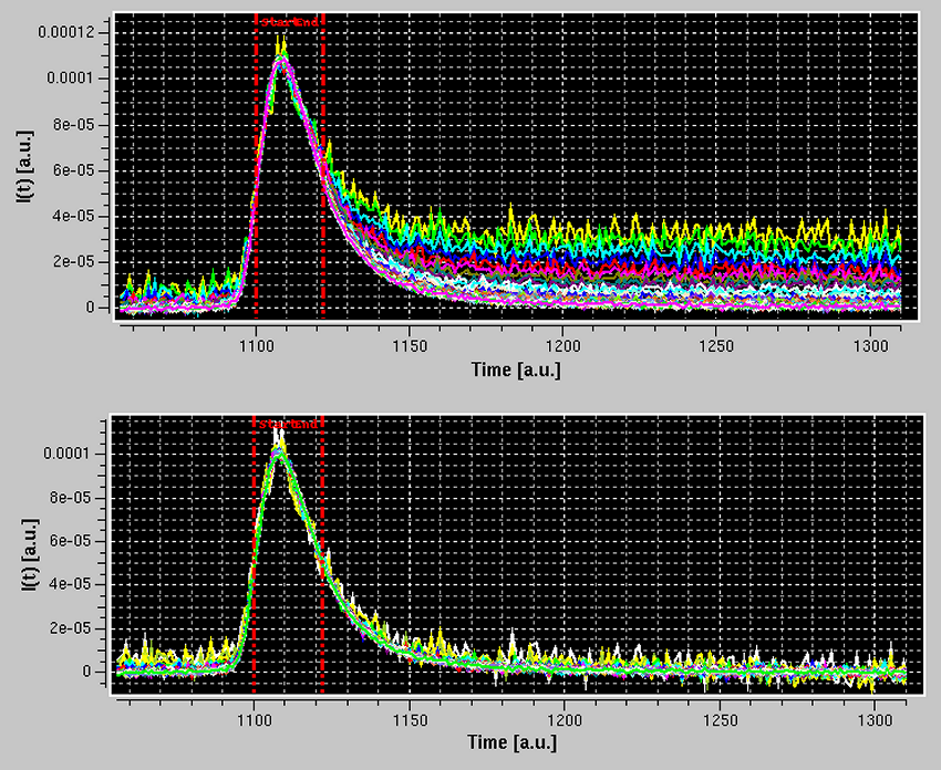
To verify what the Integral Baseline will effectively produce, Test Baseline should be launched. This will show in scroll mode every original I(t) vs. t chromatogram, a smoothed version using a Gaussian smoothing kernel of 2n+1 points (where n is set in the Options panel, with n = 3 as default), the iterations in the Integral Baseline computation (whose number is also set in the Options panel, with 5 as default), and the final, integral baseline-corrected chromatogram:

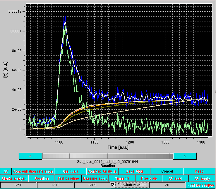
In the example shown above, blue is an original I(t) vs. t chromatogram at q = 0.00791 Å^-1, white its smoothed version with the default settings, cream, olive green, orange and pale yellow are integral baseline iterations 1, 2, 3 and 5, respectively (the 4^th iteration is not visible, completely superimposed by the 5^th), and light green is the final, integral baseline-corrected I(t) vs. t chromatogram. The Gaussian smoothing is applied to remove large oscillations in the original I(t) vs. t chromatogram, giving rise occasionally to values below the current integral baseline iteration, leading then to addition rather than subtraction in the computations. The final integral baseline is then subtracted from the original I(t) vs. t chromatogram, not the smoothed one.

As can be seen in the example above, the procedure appears to have produced a reasonable correction. All I(t) vs. t chromatograms can be checked in the Test baseline mode, which can be abandoned by pressing Cancel.

The Integral Baseline procedure can now be applied to all selected I(t) vs. t chromatograms by pressing Baseline apply. If files that failed the negative regions test within a sliding window (of 25 frames in this case) where the sum of the intensity is less than the negative of the sum of the corresponding SD values over the window are present, this message will again appear:

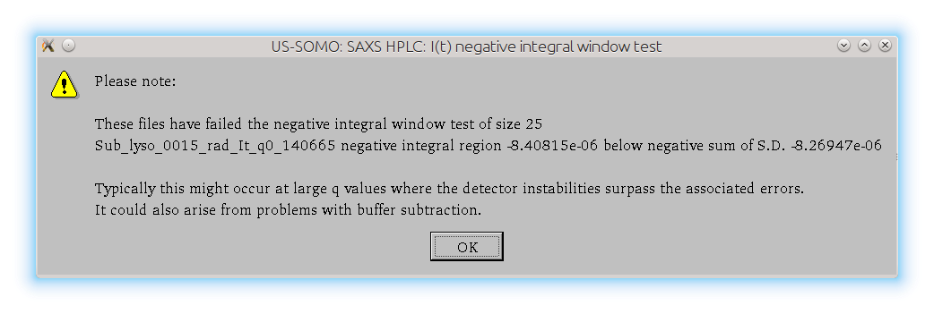
After pressing Ok, all the integral baselines will be computed and then subtracted from the I(t) vs. t chromatograms. When the overall computed change in baseline is found to be negative, no baseline correction is applied. A pop-up panel will alert the user listing the first 20 such occurences and giving the number of all the others found:

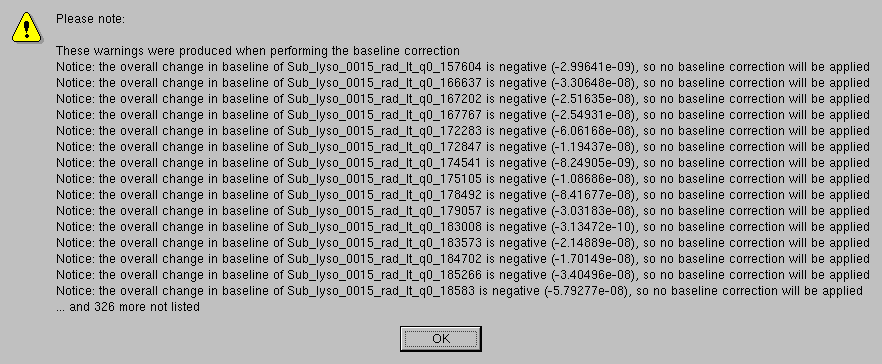
Each resulting baseline-subtracted chromatogram will have a "-bi" added after the q value and an "-s" at the end of the filename to indicate that an integral baseline subtraction was applied (if a linear baseline option is used, the first label will be "-bl"). The numerical value of the overall change in baseline and the alpha value (for an explanation alpha see here) are also added to the filename of the produced files, as shown in the Data files panel. Files where no baseline was subtracted will have a "0s" at the end of the filename:

First, the "sampling" pop-ups will appear, since in this case the sampling is not set by what was used for the Blanks:

In the following example, no sampling was applied. The sliding window size and the beginning-end of the baseline analysis region are set as with the procedure with Blanks (see above), and the Find best region button is then pressed. The CorMap results will this time be displayed with the Holm-Bonferroni checkbox automatically selected:

The second pop-up will also appear:

In respect with the analysis including a comparison with the Blanks (see above), there are two differences:

• The histogram reports the Red pair % instead of the Average Red Cluster size. This is because with the Holm-Bonferroni adjustment the formation of red cluster is severely inhibited.

• The Blanks average line is obviously absent. The cut-off to mark the histogram bars white is set to 1%. If no window reaches this level, the lowest window will be marked with a yellow color in the histogram.

The fact that the right-hand sides of the peaks are nicely superimposed after baseline subtraction validates a posteriori the procedure used to build the baseline, since for a single species the elution peaks at different q-values should be strictly proportional to each other.

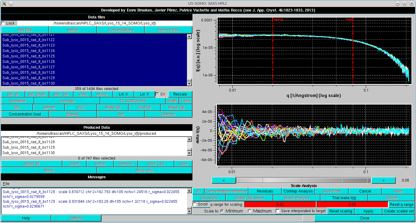
More checks of the Integral Baseline subtraction correctness can be performed using the Trial make I(q) mode. In this mode, the selected I(t) vs. t chromatograms are temporarily transposed back into I(q) vs. q frames and can be analyzed by either scaling or Guinier approximation utilities. In the example below, we have selected a subset of q-values from ≈0.008 to ≈0.21 Å^-1, and we have pressed the Trial make I(q) button:

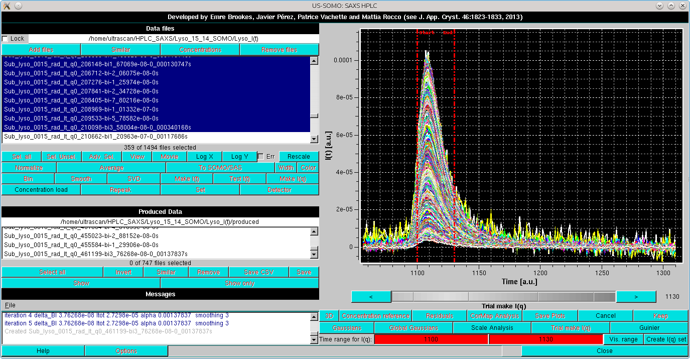
This will bring up again the gray-shades wheel-bar and change the two lowermost bars with the buttons below the graphics window. At the bottom, a Time range for I(q): label will appear, followed by two fields with red background indicating the region subjected to the Test I(q) procedure. The limits can be changed by either clicking on each red-colored field and then using the gray-shades bar-wheel at the top, or on the "<" and ">" buttons placed at its sides. Alternatively, if a region was pre-selected with the mouse, it can be applied by clicking on the Vis. range button. In this example, we have set the Time range for I(q) limits from frame 1100 to 1130.

Two operations can be then performed. Pressing the Scale Analysis button on the row above will change the layout in this way (note that, by pressing Log X and Log Y on the left-side commands panel, both axes have also been changed to log₁₀):

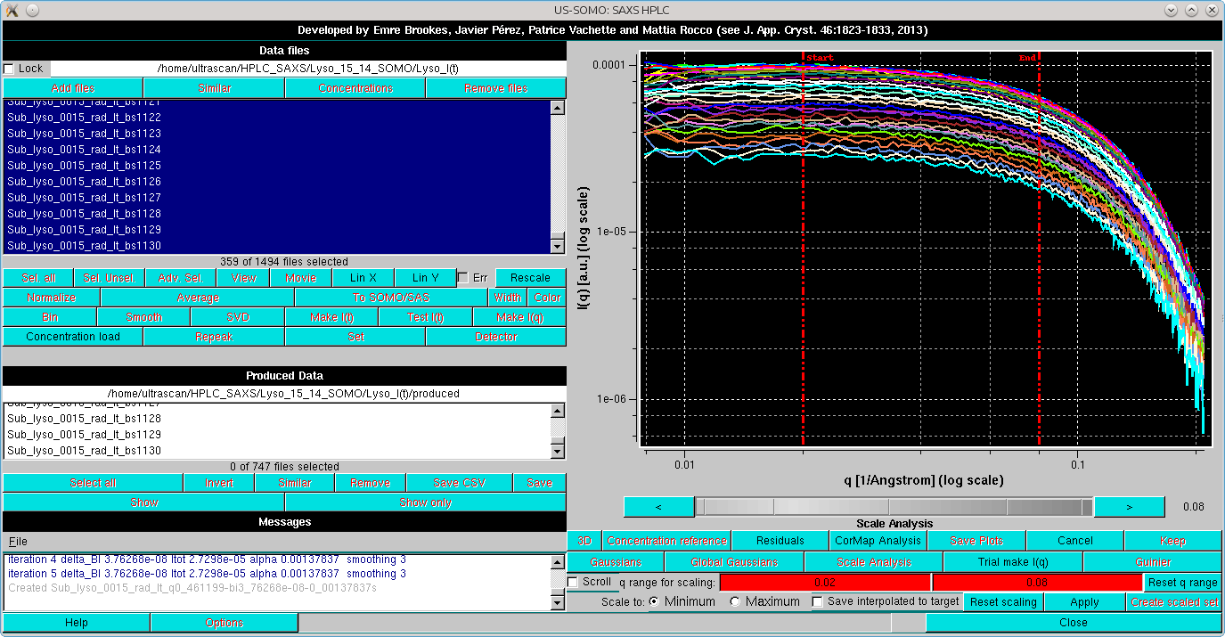
The two lowermost rows now display the tools for scaling the back-generated temporary I(q) vs. q curves on top of each other. The two red-background fields now indicate the actual q range for scaling, which can be adjusted by clicking on each field and using the gray-shades bar-wheel at the top or on the "<" and ">" buttons placed at its sides; two vertical red lines will mark the corresponding positions on the graph. The Reset q range button will re-expand the q range.
The last row contains the scaling settings/commands:

• The Scale to: round checkboxes will scale the curves to either the Minimum (default) or the Maximum values among the selected curves.

• The Save interpolated to target checkbox ensures all q or t grids of the data will be identical by interpolating each curve to the minimum or maximum intensity curve. This is a convenience tool to allow curves generated on different grids to be put on a common grid.

• Reset scaling will return to the initial situation.

• Apply will perform the scaling.

• The Create scaled set will generated an actual set of scaled data which can be then saved as files.

In the image below, the scaling has been performed on the indicated q range. The Messages panel reports the statistics of the scaling process as applied to each curve scaled on the one with the lowest intensity:

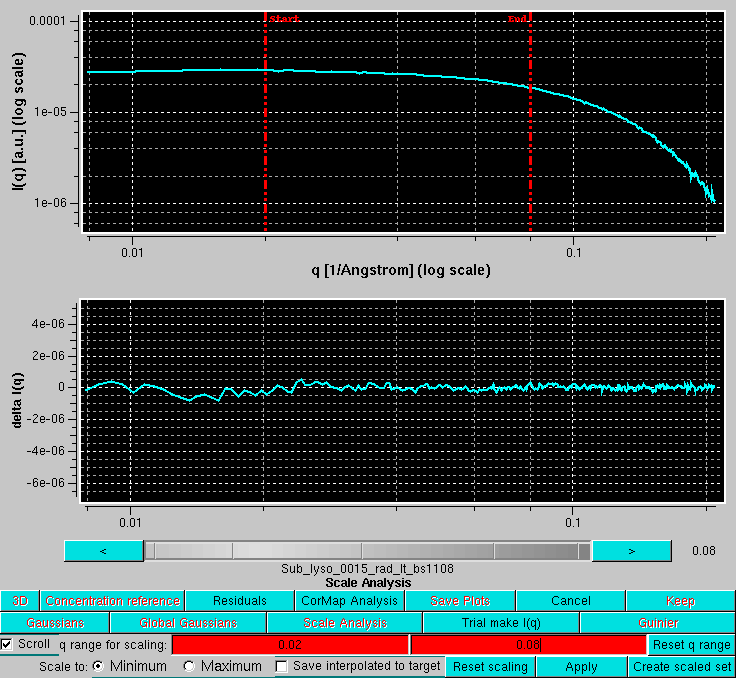
By pressing Residuals, the residuals of the scaling operation are also shown. If the Scroll checkbox is selected, the scaled files can be examined one at a time, scrolling through them using the gray-shades wheel-bar or the "<" and ">" buttons placed at its sides. The file name of the data currently shown will appear below the gray-shades wheel-bar, as shown here:

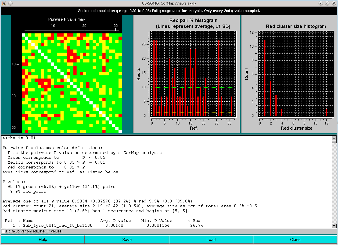
A CorMap analysis can be also performed on the scaled set by pressing CorMap Analysis. This will produce two pop-up outputs, one containg the CorMap analysis on the full q-range available:

and the other limited to the q_max value presente in the Options (0.05 Å^-1 in this case):

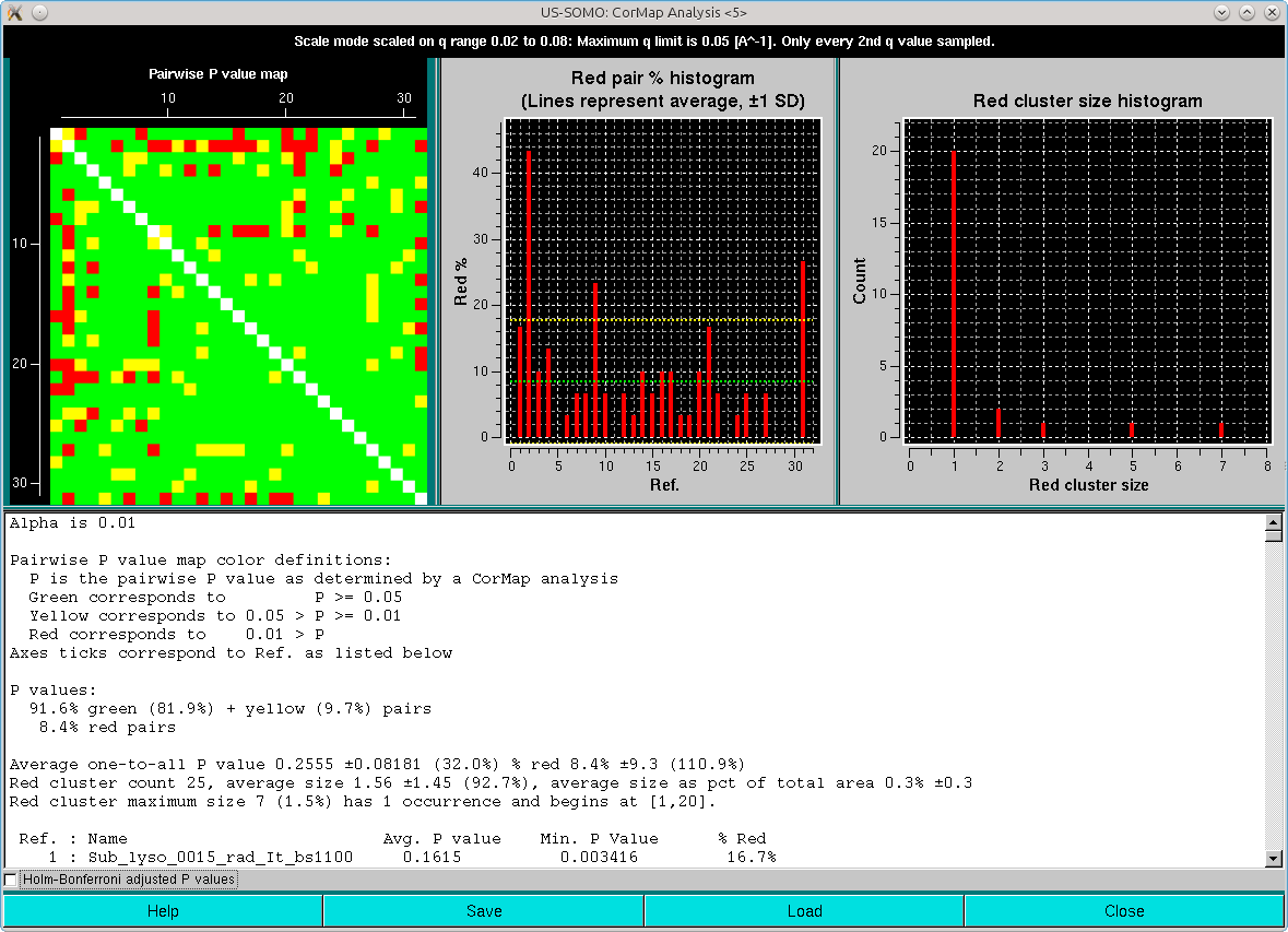
Note that one-every-other q-value has been utilized in this analysis. As can be seen, both the pairwise P-value map and the red pair % histogram indicate that with the exception of three frames of the ensemble (#2, #9 and #31, corresponding to frames #1101, #1108 and #1130), most are similar to all the others, with an overall ≈8-9% of red pairs. Limiting the lower q-values to 0.015 Å^-1 reduced this overall % red pairs count to 6% (not shown), with frames #1101 and #1130 still being substantially different from all others.

If the Holm-Bonferroni adjusted P values checkbox is selected, these will be the results:

Clearly, the combination of the one-every-other q-value sampling and the Holm-Bonferroni adjustment is over-permissive for this dataset. If the analysis is repeated without the sampling, these are the results:

In this case, similar results are obtained as with the one-every-other q-value sampling and no Holm-Bonferroni adjustment.

Pressing Cancel will completely exit from the Test I(q) mode.

Pressing Trial make I(q) will instead exit from the scaling mode only.

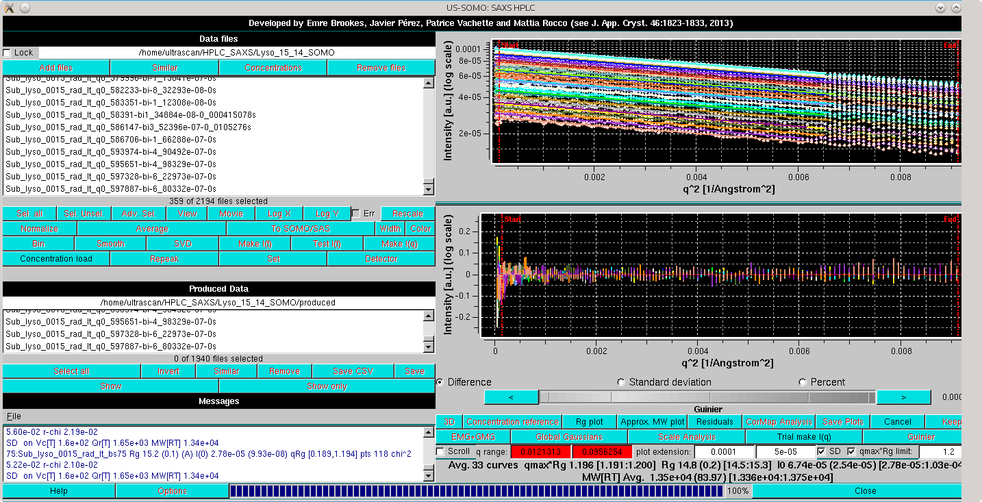
Pressing then the Guinier button will call the other test function available in the Test I(q) mode:

If the maximum q value for the currently examined I(q) vs. q dataset does not reach the MW[RT] q_max cut-off value present in the Options panel for the Rambo and Tainer approximate molecular weight calculation method (see here), a warning will appear:

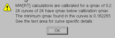
Pressing Ok will allow to proceed, showing the Guinier mode of the Trial make I(q) panel (in the case examined, the pop-up alert dit not appear, as the q_max utilized was >0.2 Å^-1):

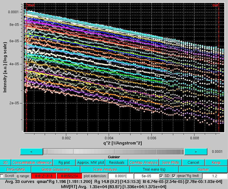
The lowermost row now carries the tools necessary to perform a Guinier analysis on the back-generated temporary I(q) vs. q curves:

• The q range: fields (red background) indicate the q range currently selected. By clicking on each one and using the gray-shades bar-wheel at the top or the "<" and ">" buttons placed at its sides, the q-range can be changed.
  
• The plot extension: fields provide a q range extension of the Guinier and Residuals plots, allowing additional q range before (left box) and after (right) the Guinier range to be shown. By clicking on one and using the gray-shades bar-wheel at the top or the "<" and ">" buttons placed at its sides, the q-range extension can be changed.
  
• The SD checkbox controls if the linear regressions for the Guinier analyses are carried out with SD weighting (default: checked).
  
• The qmax*Rg checkbox and its associated field enable a sequential routine which examines, starting from the higher q value utilized in the regression (q_max), if the product q_max*R_g is ≤ the limit set in the apposite field (the default value is set in the Options panel). If the products exceeds the limit, that q_max value is dropped, and the regression is repeated utilizing the next lower q value. The test is repeated until a q_max value satisfying the q_max*R_g ≤ set limit is found. It is highly advisable to deselect this checkbox before manually changing the q range fields, and to re-select it afterwards, otherwise the program will continuously repeat the q_max*R_g routine while the limits are manually moved.

• The number of curves used (Avg. xx curves);
  
• The average qmax*Rg (where qmax is the maximum q value included in the Guinier analysis), with the range in square brackets;
  
• The average Rg, with the SD in round brackets and the range in square brackets;
  
• The average intensity extrapolated at 0 scattering angle I0, with the SD in round brackets and the range in square brackets.
  
• In the line below, an approximates molecular average molecular weight, MW[RT] is reported, together with its SD (in round brackets) and range [in square brackets], based on the method of Rambo and Tainer (Accurate assesment of mass, models and resolution by small-angle scattering. Nature 496:477-481, 2013). If the available q-range is below that required by the method, a warning message appears in the Messages area.

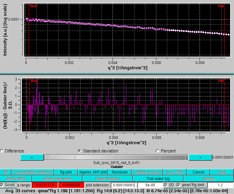
The residuals of each linear regression can be seen by pressing Residuals:

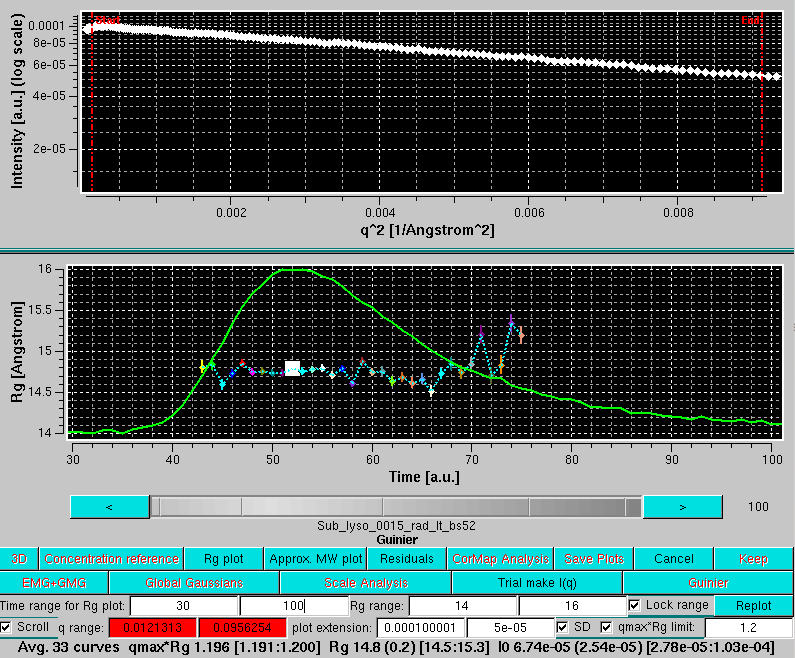
Note how the average Rg recovered for this extended set, 14.8±0.2 Å, compares well with the 15.0 Å that can be calculated from the lysozyme average NMR structure (1E8L.pdb) using the WAXSiS server (http://waxsis.uni-goettingen.de/).

As with the scaling option, every individual Guinier plot can be visualized by selecting the Scroll checkbox and using the gray-shades wheel-bar:

At this point, a plot of the Rg values across the chromatogram together with a typical I(t) profile (continuous green curve) can be shown by pressing Rg plot:

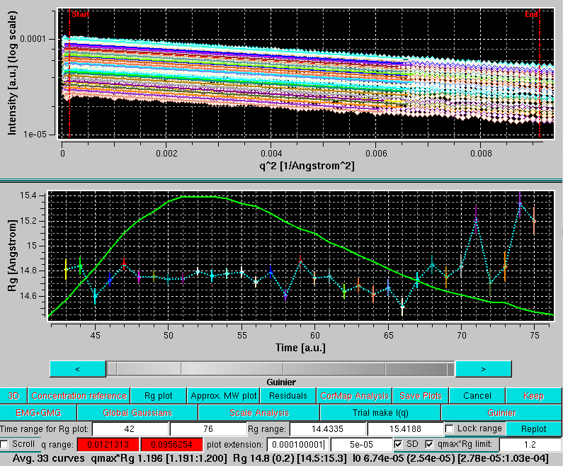
A new row will appear below the graphics window, with these fields:

• Time range for Rg plot: with its two fields. Clicking on each one and using the gray-scale bar-wheel at the top or the "<" and ">" buttons placed at its sides will allow to expand or restrict the Time axis (by default, the original time range is shown).
  
• Rg range: with its two fields. Clicking on each one and using the gray-scale bar-wheel at the top or the "<" and ">" buttons placed at its sides will allow to expand or restrict the R_g range. The default is governed by the actual R_g with error bars range with an additional empty space of 2.5% of the total range added to the lower and upper R_g limit.
  
• The Lock range checkbox if selected will maintain the actual shown R_g range. Pressing the Replot button will replot the data keeping the selected R_g range and maximizing the I(t) profile within the selected time range limits.
  

The scroll capability can also be activated in this mode, and the currently selected Guinier plot will be highlighted in the R_g plot:

Likewise, plots of the approximate molecular weight calculations can be shown by pressing the Approx. MW plot button:

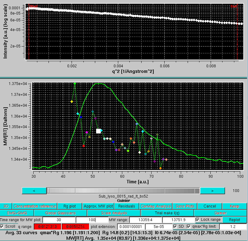
Pressing Test I(q) button will bring back the main options of this utility.

Pressing the Cancel button will exit the Test I(q) utility.

If Gaussian analysis is not required, a series of I(q) vs. q frames can be re-created at this stage from the baseline-corrected data by pressing the Make I(q) button.

This document is part of the UltraScan Software Documentation distribution.
Copyright © notice.

The latest version of this document can always be found at:

http://somo.aucsolutions.com

Last modified on June 30, 2024.