
| |
Manual |
This US-SOMO module was originally conceived for the analysis of HPLC-SAXS data, in particular from size-exclusion chromatography (SEC). From the US-SOMO July 2024 intermediate release, it has been renamed HPLC/KIN to reflect the enhancements that were made to deal with kinetics-derived data, which are similar in certain aspects to the on-line chromatography-derived data. The vast majority of this Help will still extensively deal with the treatment of SEC-SAXS data.
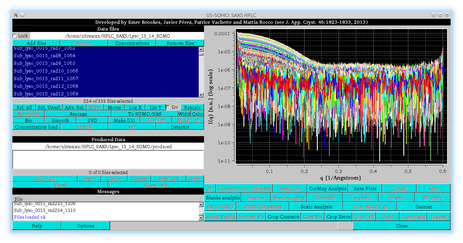
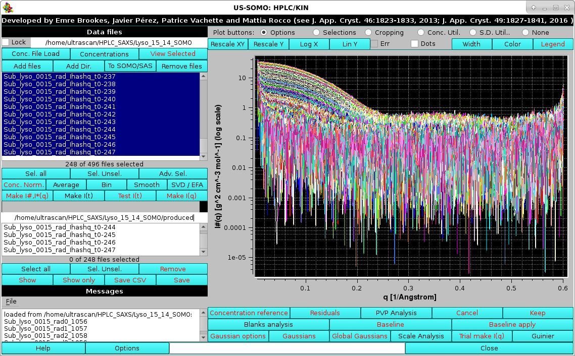
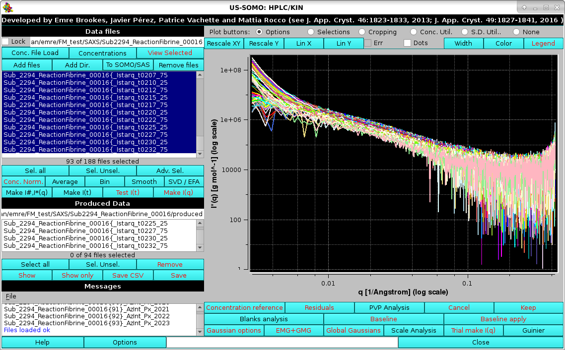
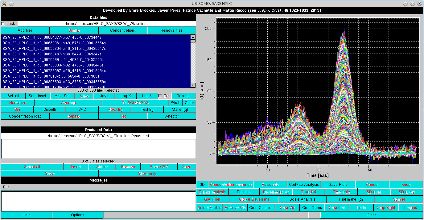
In the image above, the main panel of the HPLC/KIN module is shown. The buttons with the black labels are the ones currently active, the ones with the red labels become active when allowed by the processing/visualization stage. The graphics panel shows a collection of HPLC-SAXS log10[I(q)] vs. q SAXS data frames (points with 0 or negative values are automatically omitted from the visualization only) for a chicken egg-white lysozyme chromatographic separation on a Agilent BioSec-3 (3 μm particle size, 300 Å pore-size) 4.6 × 300 mm column, eluted with Hepes 50 mM, NaCl 100 mM, pH 7. Note the permanent upturn at very small q-values, due to biological material aggregated by the intense X-ray beam on the capillary cell walls under these far from optimal experimental conditions. While this kind of problem should be (and has been) preferentially dealt with at the experimental level, we use this dataset to demonstrate the potential for correcting data still presenting such an issue.
The left side of the window is divided in three sections, labeled "Data files", "Produced Data", and "Messages". By clicking on these labels, the corresponding panel below each label will disappear, allowing for an expansion of the remaining other panel(s). If every panel is made to disappear, the main graph will expand to cover the full size of the HPLC/KIN module window. By clicking again on the labels, the corresponding panels will be restored.
On the top left panel (Data files) there are seven buttons:
 |
 |
Below the window with the loaded files listing there is a second section of buttons:
 |
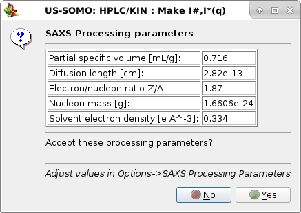 |
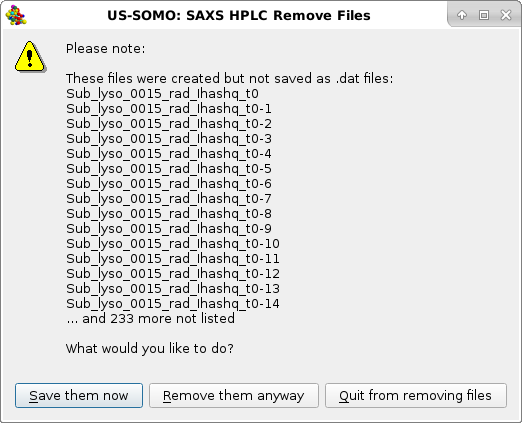
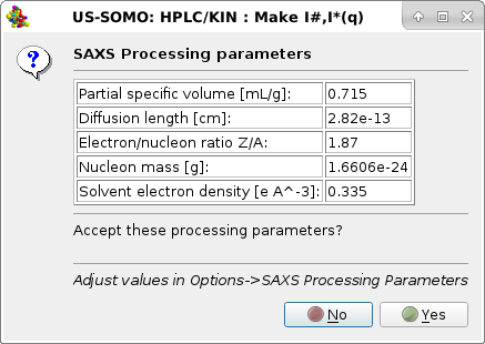
listing the SAXS processing parameters as stored in the SAXS Processing parameters sub-module of the HPLC/KIN Options module. If these parameters are deemed not correct for the sample being analyzed, pressing No will stop the operation, otherwise pressing Yes the I(q) vs. q data will be later on internally converted to I#(q) or I*(q) vs. q, and another pop-up panel will appear:
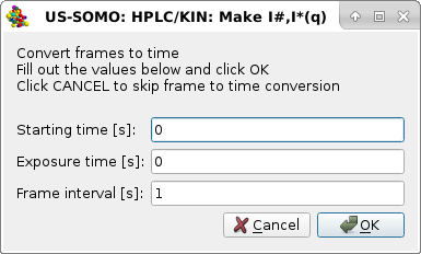 |
asking for optionally converting the frame numbers to times with the default values shown in the image. The Starting time [s] can be left to "0" (the choice for kinetic data if they have been already trimmed to the starting point of the reaction), or it allows to correctly assign the elution time of the first frame for SEC-SAXS data, which are usually not recorded until the beginning of the sample elution from the column. The Exposure time [s] (default "0") can also be optionally inserted in the second field, in which case be careful to correctly enter the Frame interval [s] (default "1") in the third field. For instance, if the exposure time is 0.01 s, a frame interval of 0.99 s will then produce a step of 1 s between the frames.
Pressing Cancel will avoid converting frame numbers to times, pressing OK will perform this operation. Regardless of the choice (we hit Cancel in this example), a third pop-up panel will appear:
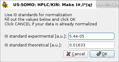 |
this time asking if a normalization of the I(q) data should be performed. The values shown for the experimental and theoretical I0 of the standard are also taken from the SAXS Processing parameters sub-module of the HPLC/KIN Options module, but they can be modified here.
Pressing Cancel will avoid normalizing the I(q) data (the usual choice since nowadays data are given to the user already normalized), pressing OK will perform this operation (we hit OK for this example as the data were not already normalized). A fourth pop-up panel will then appear:
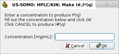 |
in which a solute global concentration [mg/mL] can be entered. Entering a concentration is appropriate for kinetic or batch data, where it is expected to remain constant for all frames. For chromatographic data (as in this case), the solute concentration varies frame-to-frame, and can be later asessed from UV or RI monitors data.
Pressing Cancel will then produce I#(q) vs. q frames (as in this example), while entering a concentration and pressing OK will produce I*(q) vs. q frames, as indicated in the final pop-up panel:
 |
Pressing OK the procedure completes, and the I#(q) or I*(q) vs. q produced data will be shown in the Data files panel, automatically selected only and thus appearing in the graphics window with the correct units posted on the y-axis label:
 |
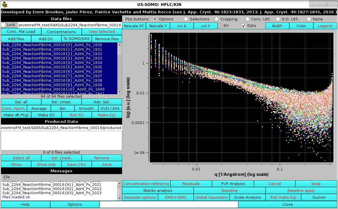
As a kinetics data processing example, we load SAXS data on a fibrin re-polymerization experiment, where fibrin monomer obtained from solubilization of a fibrin clot with sodium acetate 100 mM, pH 4.6, and purified by SEC on a preparative column, was mixed it in a 1:1 ratio with Tris 65 mM, NaCl 100 mM, pH 12.3, restoring near-physiological conditions of pH ∼7.4. The reaction mixture was sequentially injected into a Multi-Angle Light Scattering (MALS) detector and in the SAXS capillary. SAXS frames were recorded every 2.5 s with a sample-to-detector distance of 2.56 m (Rocco, Thureau, Pérez, et al., manuscript in preparation):
 |
After entering the appropriate parameters for this sample/buffer in the SAXS Processing parameters sub-module of the HPLC/KIN Options module, we press Make I#,I*(q), and the pop-up will appear:
 |
listing the new SAXS processing parameters. Pressing Yes the I(q) vs. q data will be later on internally converted to I#(q) or I*(q) vs. q, and the second pop-up panel will appear:
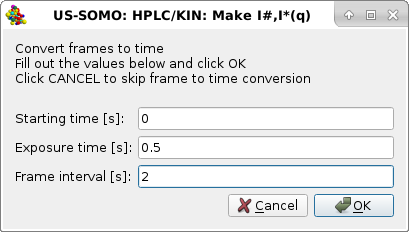 |
We leave the Starting time [s] "0" as these kinetic data were collected immediately after injection. We set the Exposure time [s] to 0.5 s and the Frame interval [s] t0 2 s. Pressing OK will perform this operation, and the third pop-up panel will appear:
|
asking if a normalization of the I(q) data should be performed. We press Cancel since the data were already normalized at the beamline. The fourth pop-up panel will then appear:
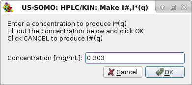 |
in which a solute global concentration [mg/mL] can be entered. We enter 0.303 mg/mL, appropriate for these kinetic data, where it is expected to remain constant for all frames. Pressing OK will produce I*(q) vs. q frames, as indicated in the final pop-up panel:
 |
Pressing OK the procedure completes, and the I*(q) vs. q produced data will be shown in the Data files panel, automatically selected only and thus appearing in the graphics window with the correct units posted on the y-axis label:
 |
These data can be then joined with MALS-derived data in the MALS+SAXS module (see here).
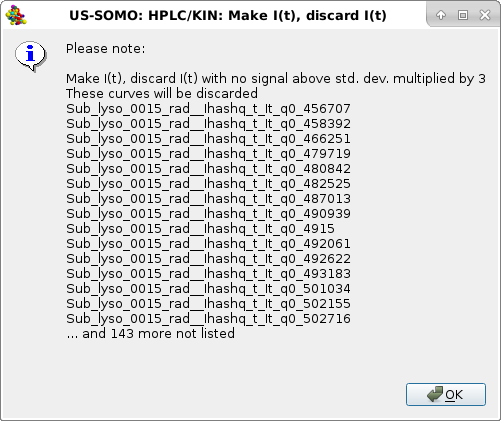 |
In this case, relatively few files did not pass this test, all in the high q-range. Pressing OK will allow the process to proceed, and a second test is performed, the negative integral window test (with a sliding size of 25 points):
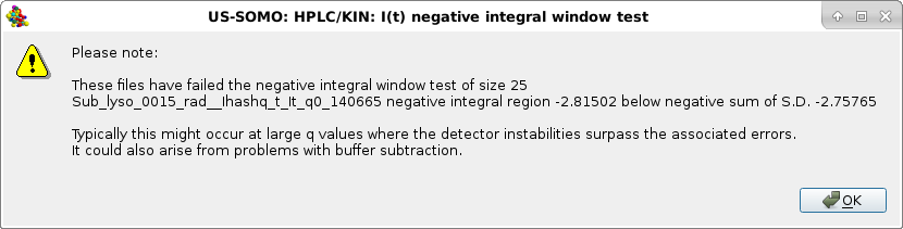 |
Here, just one file failed the test (see here for a full explanation of this test's significance). Pressing OK will allow the process to complete:
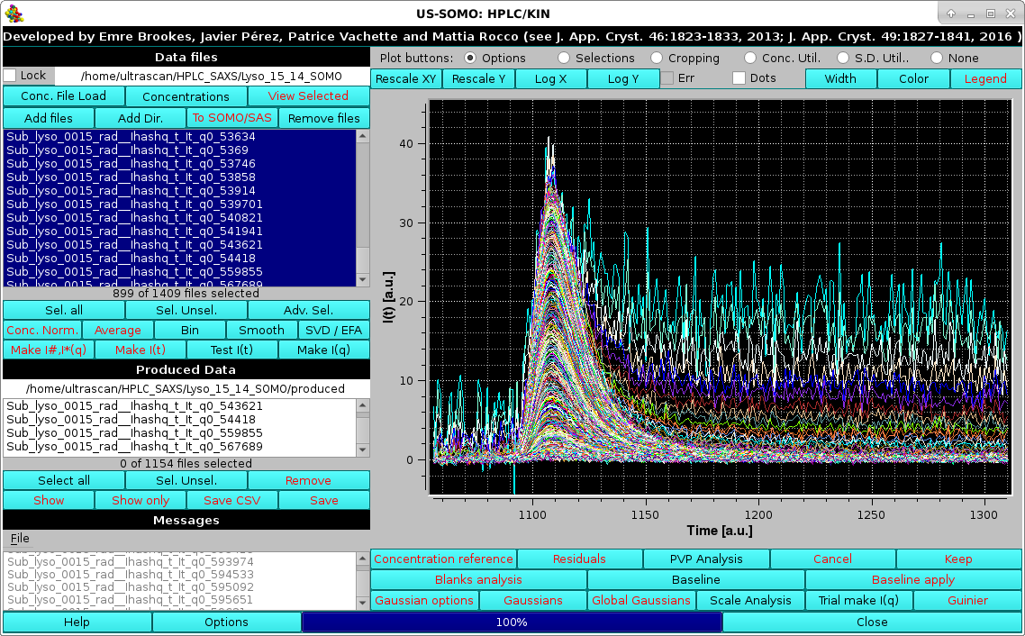 |
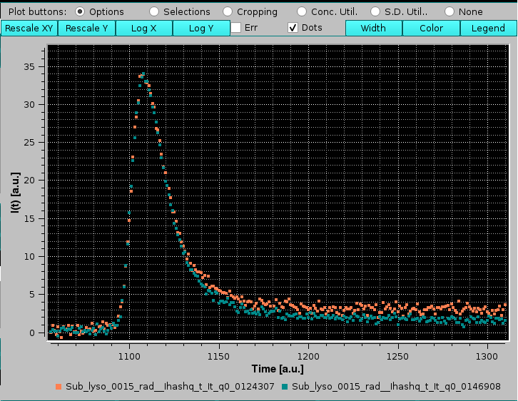
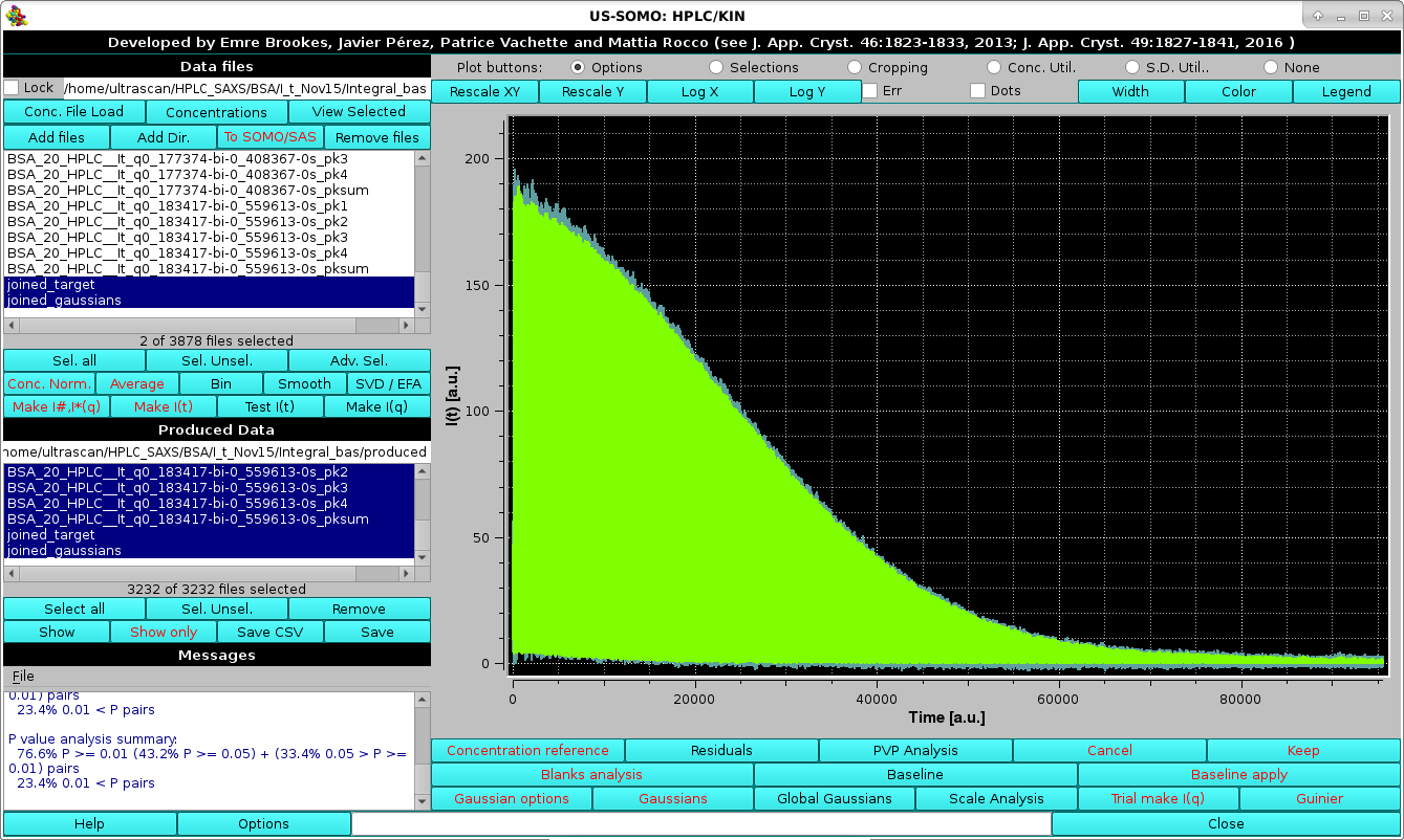
resulting in the data been shown as a series of I#(t) vs. t chromatograms (automatically selected only), one for each scattering angle, whose value is reported in the generated files names with the extension "qx_xxxxx", where "x_xxxxx" is the q-value with "_" replacing the decimal point. Visual inspection of the I(t) vs. t chromatograms can already hint at problems, such as in the lysozyme data here used as an example. In this case, it is evident that many I(t) vs. t chromatograms starting from the low-q region do not return to pre-peak elution baseline intensity values. Most likely, this is due to capillary fouling, and without proper correction these data would be mostly useless. For this, and for less evident cases, an Integral Baseline correction procedure has been devised (see below and here for a full description of this utility).
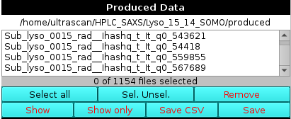
The file names of produced data are shown in the Produced Data panel to the centre-left, and can be selected and saved to files using the appropriate buttons below it.
 |
 |
The bottom line of this module contains the Help, Options, and Close buttons, with in between a progess bar showing in blue color and with a numeric % value the advancement of the currect action:
 |
On pressing Options, a pop-up panel will be shown:
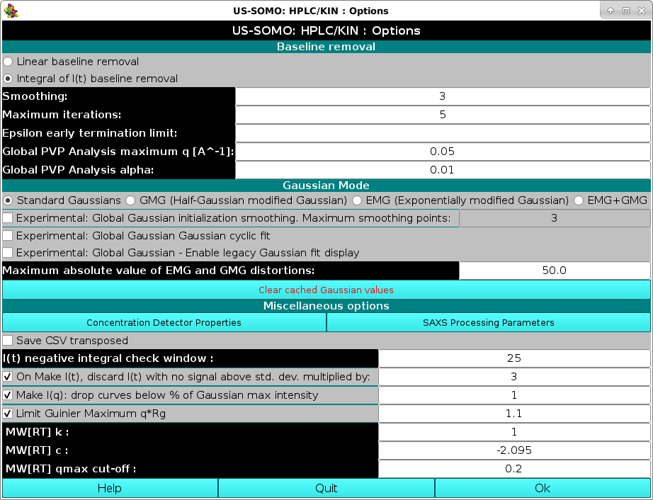 |
See here for a description of this module.
On the top of the graphics window there is a row of round "Plot buttons:" checkboxes each one controlling the showing of a series of buttons:
 |
The Options checkbox will enable these buttons:
 |
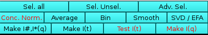
The Selections checkbox will enable these buttons:
 |
 |
When a part of the graph is selected using the mouse/left button, the buttons become all available (only Crop Zeros and Crop Common are available when files are just displayed after selection).
 |
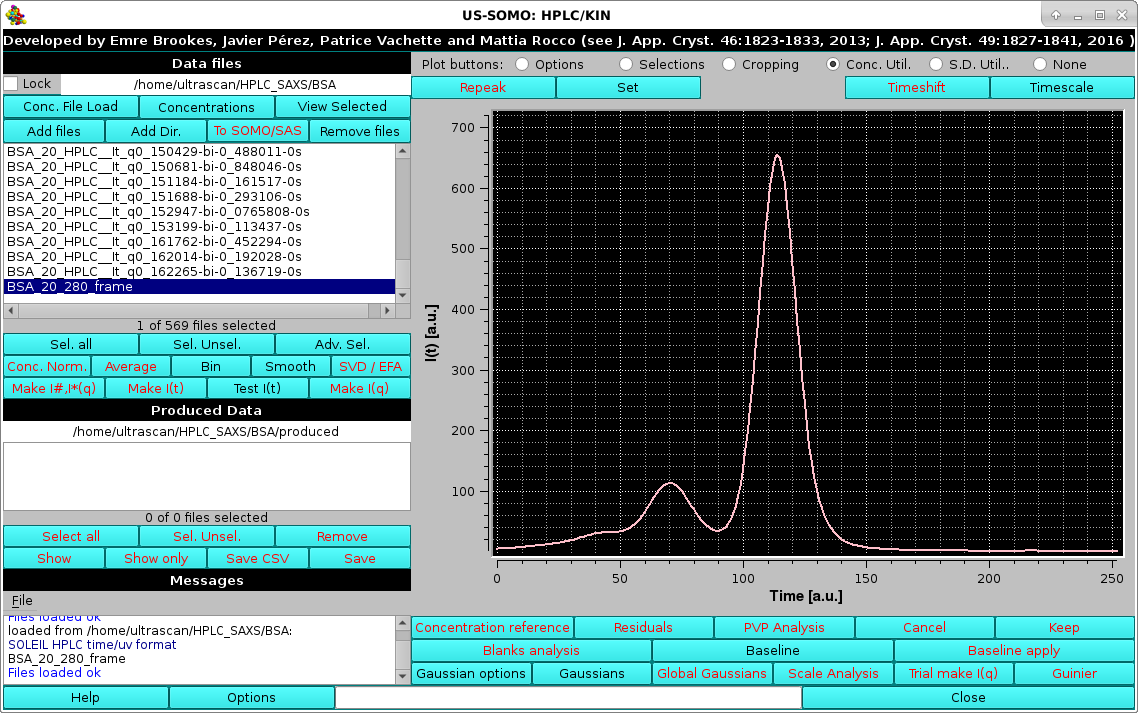
They are used to deal with chromatography data coming from a concentration detector, such as absorbance (UV-Vis) or refractive index (RI). These data are usually on a diffent intensity scale, and time-shifted because of the placement of these detectors either before or after the SAXS cell. To deal with these problems, we need first to scale the concentration-associated chromatogram to a SAXS I(t) vs. t chromatogram at a q value, and then to time-shift it to align it in the time domain.
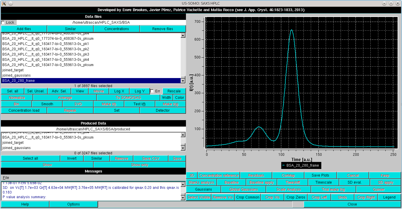
To demonstrate these procedures we employ a bovine serum albumin (BSA) SEC-SAXS run using two 7.8 × 300 mm ID columns packed with hydroxylated polymethacrylate particles (TSK G4000PWXL, 10 µm size, 500 Å pore size, and G3000PWXL, 6 µm size, 200 Å pore size, Tosoh Bioscience, Tokyo, Japan) connected in series, protected by a 6 × 40 mm guard column filled with G3000PW resin (Tosoh). The data presented capillary fouling evidence, and were thus subjected to Integral Baseline correction (not shown). The concentration-associated data were an absorption profile at 280 nm collected with a DAD (Diode Array Detector).
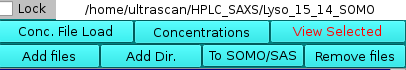
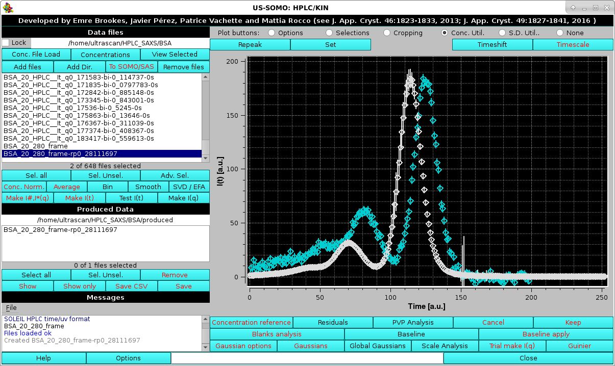
The concentration data are first loaded with the Conc. File Load button (see here) and then selected:
 |
Then, usually a low-q, high-intensity but low-noise I(t) vs. t chromatogram is also selected:
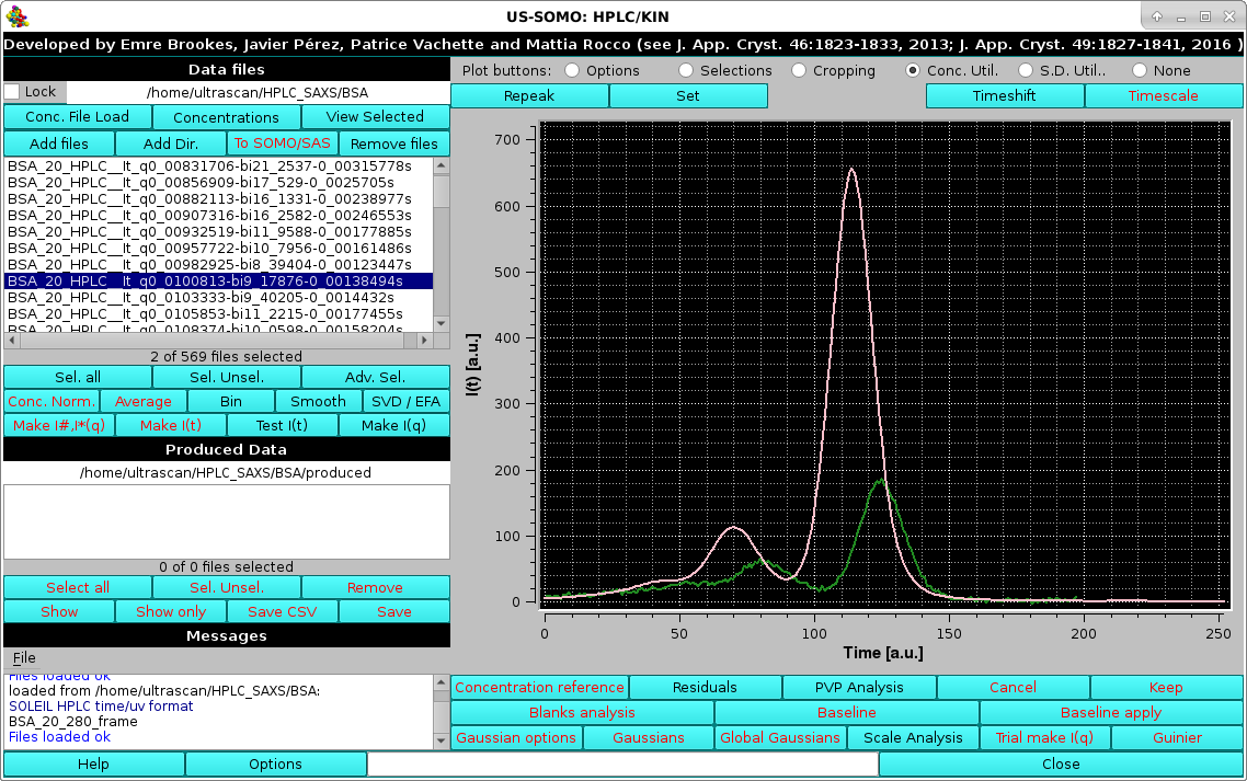 |
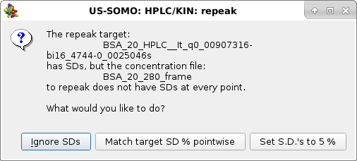
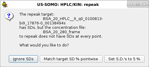 |
Usually the SD are ignored by pressing the first option presented, but the module offers two other alternatives, Match target SD % pointwise and Set S.D.'s to 5% (these two choices could be useful in the Gaussian decomposition procedure if less stringent constraints are sought for the concentration associated data). Whatever the choice, the repeak operation affects the data, a new file is generated with "rp" extension and the scaling factor, which will be used to re-generate the proper intensity scale when needed, added at the end of the filename:
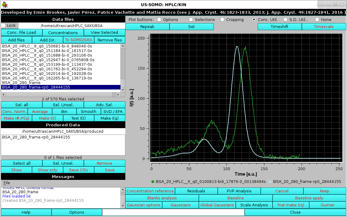 |
At the same time, another pop-up panel will ask if you want to "*Set*" (see below) the repeaked concentration file:
 |
In this case the answer will be No, since the two chromatograms are still time-shifted one in respect to the other.
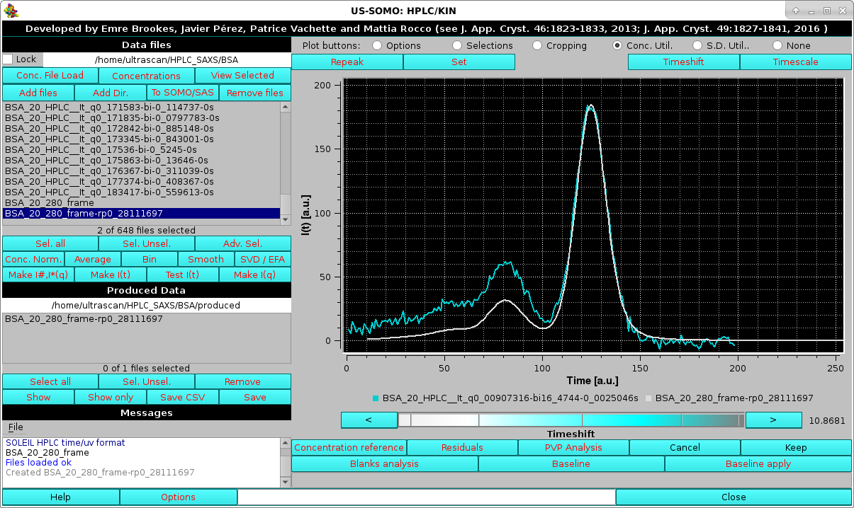
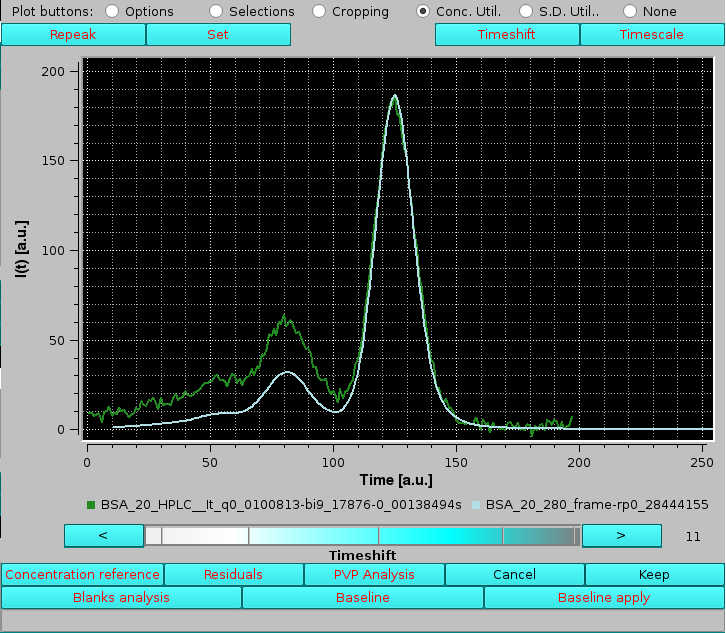 |
If this traslation doesn't occur automatically, it can be initialized by acting on the "<" and ">" buttons at the extremities of the cyan-shades bar-wheel below the graphics window. The resulting traslation of the concentration-associated dataset can be either refused by pressing Cancel, or accepted by pressing Keep using the buttons placed below the graphics window. On pressing Keep, another pop-up panel will show up:
 |
Pressing No will defer this important decision, pressing Yes will already define this repeaked, time-shifted concentration-associated chromatogram as the source of frame-by-frame concentration values for the SAXS data:
 |
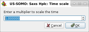 |
were a multiplying factor can be entered. For instance, if the time units of the concentration data were minutes, and of the SAXS data were seconds, entering "60" and pressing Ok will bring the concentration data on the same time units as the SAXS data. This operation, if needed, should be done before any other in this panel. Pressing Cancel will abort this operation.
The S.D. Util checkbox relates to another feature present in the US-SOMO HPLC/KIN module, an alternative way of estimating the errors associated with the SAXS data. This might become useful if no errors have been already associated with the experimental data, or if their reliability is questionable.
The method is based on the assumption that the fluctuations of the signal at the baseline level are a good representation of the error associated with the data an any other point along each I(t) vs. t chromatogram. Therefore, by estimating the average fluctuations in flat regions of the chromatogram, a constant SD value can be associated with every datapoint in that particular chromatogram. Obviously, different chromatograms will have different values for their respective constant SD.
Two buttons will become availble on selecting the S.D. Util checkbox:
 |
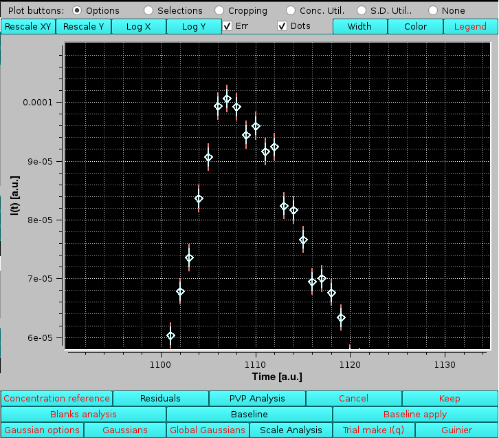
For this example, we use an Integral Baseline corrected I(t) vs t chromatogram produced from the lysozyme SEC-SAXS data employed at the beginning of this Help section (see here for a full description of this utility).
The actual SD associated with it can be visualized by selecting the Err checkbox in the Options menu as described above:
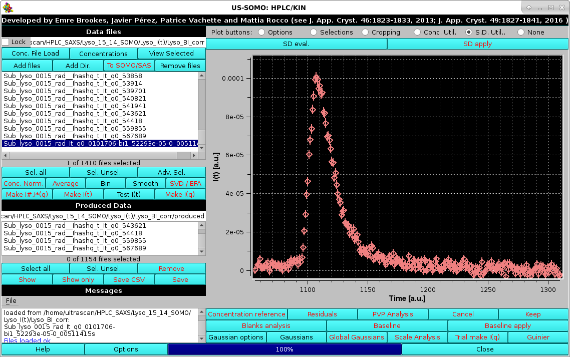 |
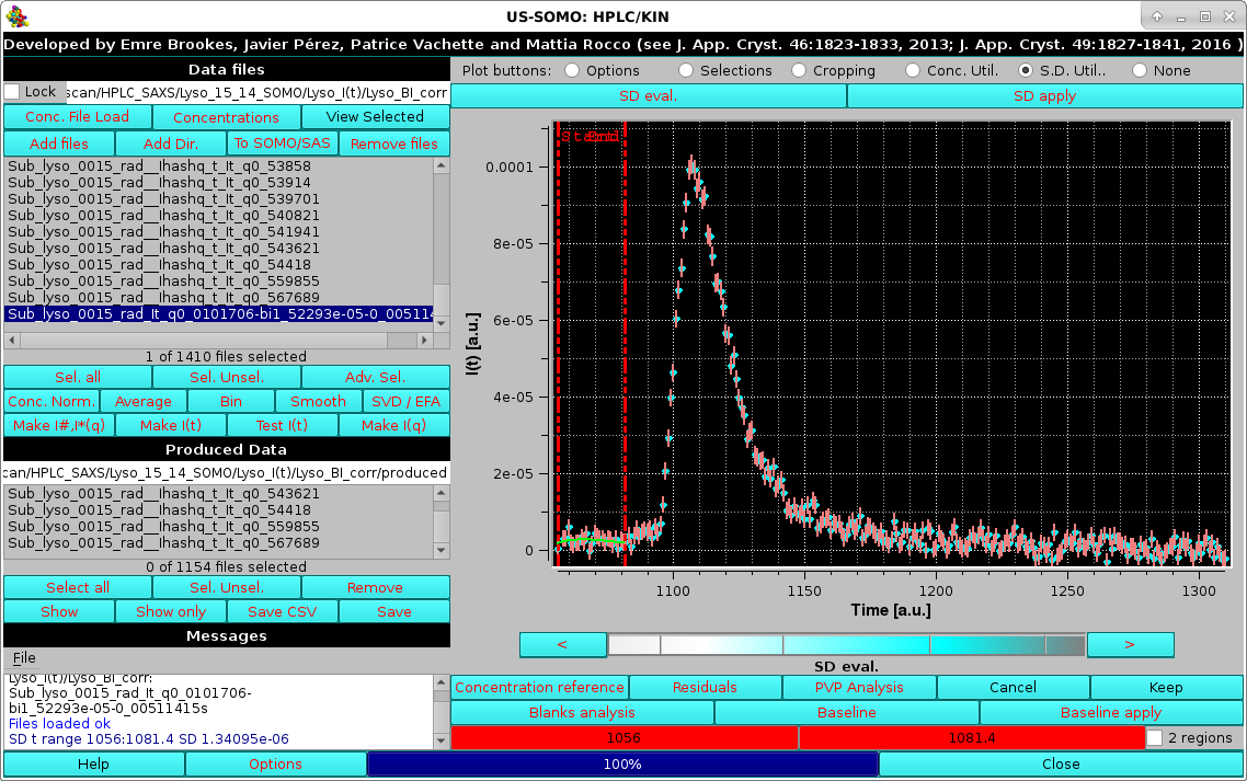 |
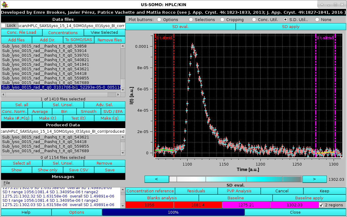 |
The SD evaluation is carried out by fitting the data included between each zone with a 3rd degree polynomial, and taking the RMSD of the fit as the SD. If two regions are chosen, the final SD will be an average between the values computed from each region. These values are reported on the Messages section.
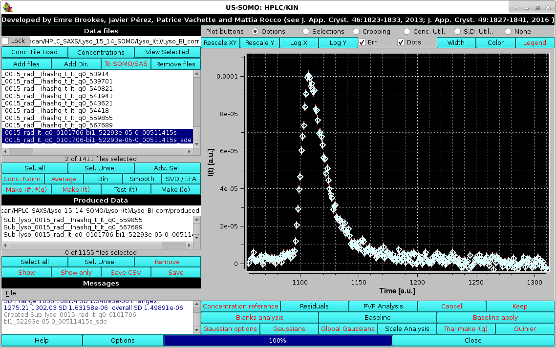 |
A zoom-in of the main peak region highlights how the two SDs are very close to each other:
 |
demonstrating that the assumptions taken for this alternative SD evaluation produce SDs which are very similar to the ones that have been associated to the original SAXS data using a Poisson distribution. The main difference is that the original SDs vary slightly with the intensity for each I(t) vs. t chromatogram, while the baseline fluctuations method produces constant SD values for each I(t) vs. t chromatogram.
Below the US-SOMO HPLC/KIN module graphics panel there are a series of buttons for performing several operations on the files displayed, some of which will become available only when multiple files are selected, or a region of the graph is zoomed, while others will become available only when single files are selected:
 |
Note: some buttons are not always visualized, but will appear in place of others when some functions are called, such as in the SD evaluation procedure described above.
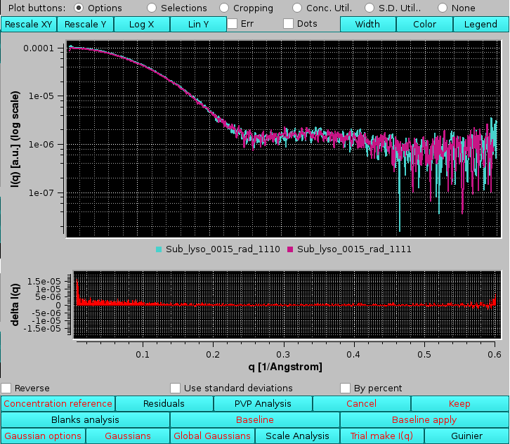 |
Selecting the Reverse checkbox will inverted the order of comparison and thus the sign of the differences. Selecting the Use standard deviations checkbox will weight the residuals by the associated SD of each point:
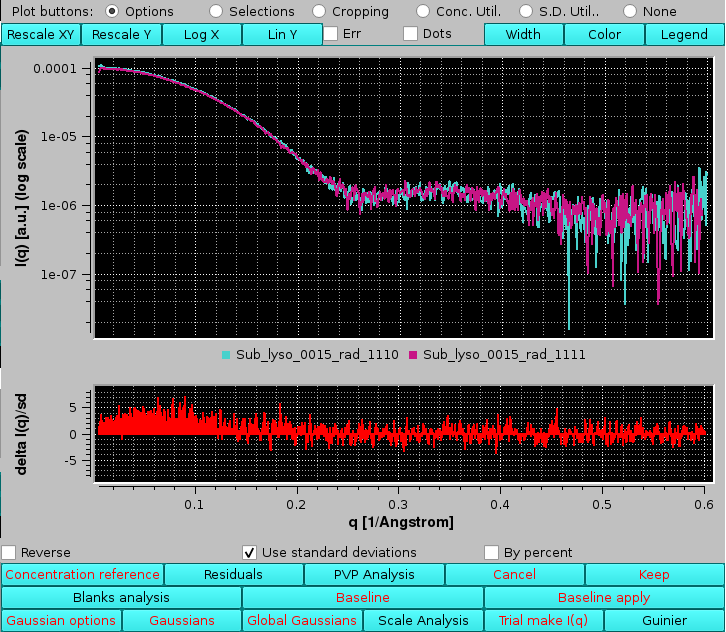 |
Selecting instead the By percent checkbox the residuals will be plotted as % values:
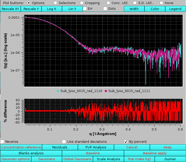 |
The residuals plot can be toggled off by pressing again Residuals.
Gaussian decomposition of not baseline-resolved peaks is another utility present in the US-SOMO HPLC/KIN module. Decomposition with symmetrical Gaussian functions will be first described using a bovine serum albumin (BSA) SEC-SAXS run using two 7.8 × 300 mm ID columns packed with hydroxylated polymethacrylate particles (TSK G4000PWXL, 10 µm size, 500 Å pore size, and G3000PWXL, 6 µm size, 200 Å pore size, Tosoh Bioscience, Tokyo, Japan) connected in series, protected by a 6 × 40 mm guard column filled with G3000PW resin (Tosoh). The data presented capillary fouling evidence, and were thus subjected to Integral Baseline correction (not shown).
Before proceeding to Gaussian analysis (whose theory can be seen here), a SVD analysis could be useful. In SVD analysis, the number of significant singular values in the decomposition should be equal to the number of components in the data, and thus to the minimum number of Gaussians required to accurately reconstruct the data (see here).
Three buttons control the Gaussian decomposition procedure in the HPLC/KIN module of US-SOMO: Gaussian options, Gaussians, and Global Gaussians.
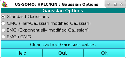 |
It also offers the possibility of re-initializing the Gaussian analysis by pressing the Clear cached Gaussian values button. For this demonstration, we will leave the default Standard Gaussian checkbox selected. Quit will exit from this pop-up without retaining any changes, Ok will exit maintaining any changes made.
By default, the US-SOMO HPLC/KIN module will consider symmetrical Gaussians, but distorted Gaussian functions are also availble and can be selected from the Gaussian Options menu (see above). The choice must be done before starting the following procedure. An example of a data processing with non-symmetrical Gaussians is presented here.
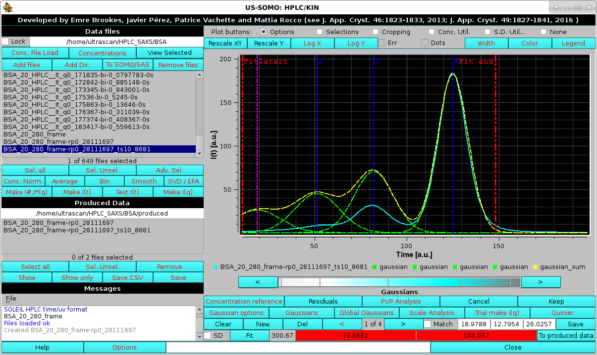
On pressing Gaussians, two new rows of buttons/fields and a checkbox will appear at the bottom of the graphics window, together with two vertical red dashed lines indicating the Fit start and Fit end points of the Gaussian fitting region, whose directly editable values (default: at the beinning and end of the available data) appear in the two red-background fields in the bottom row:
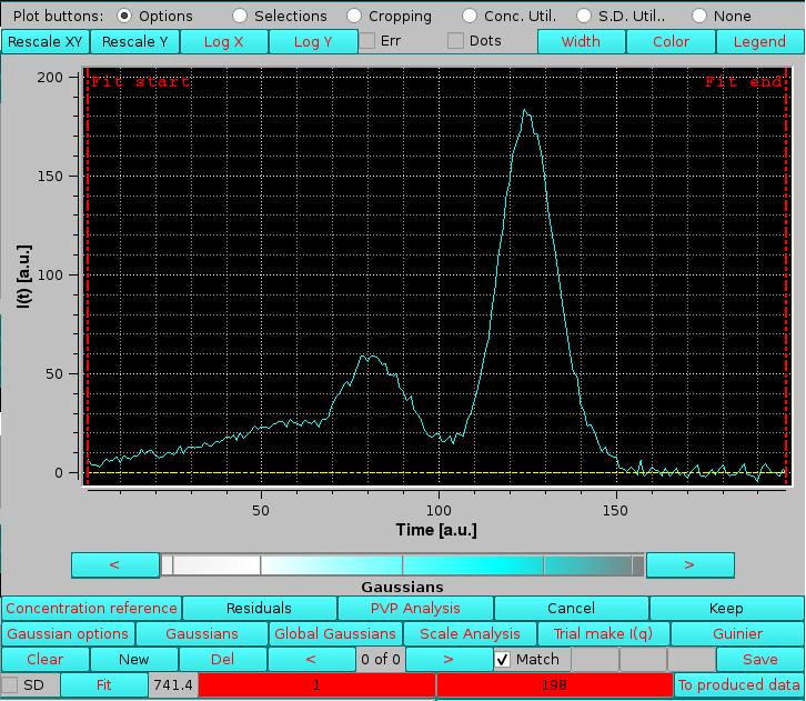 |
If a previously-generated set of Gaussians was present or loaded from file, the Gaussians will show up under the peak(s) together with vertical lines indicating their centers, such as in the example shown below, where also the Fit end vertical line has been moved to a new position from the default settings:
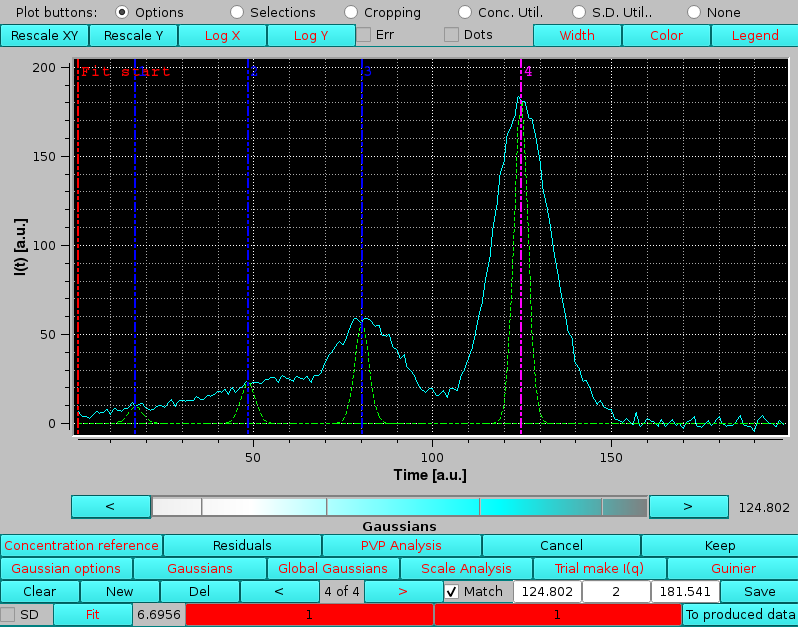 |
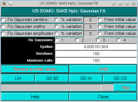
See here for a description of the Fit module.
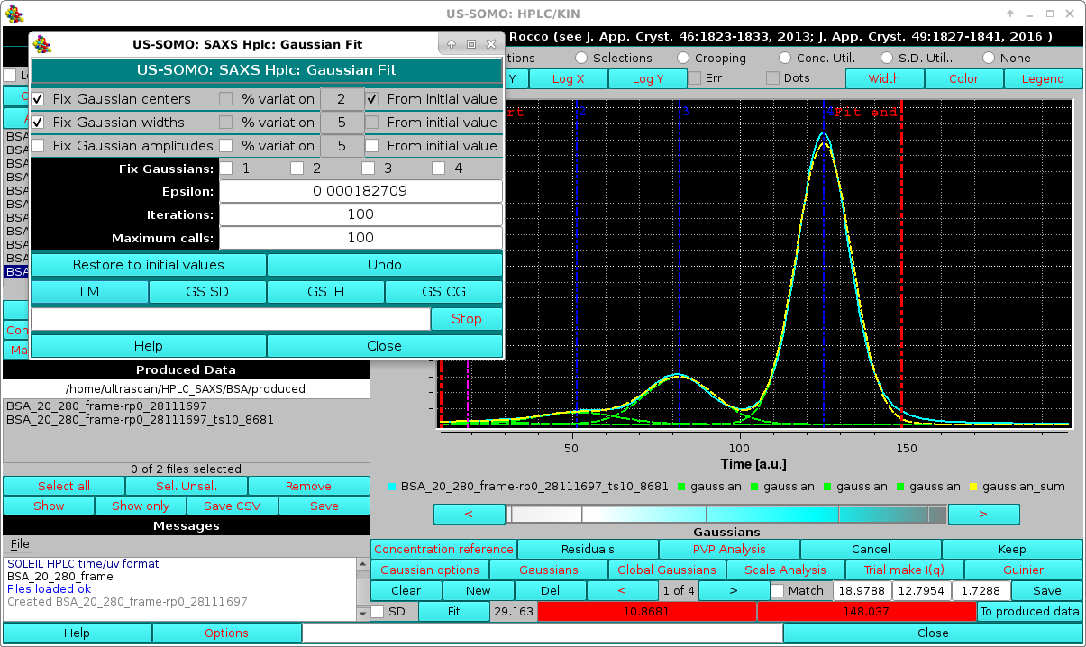
In the first cycle of iterations, it is best to keep the original centers fixed:
 |
In the example shown, a not well-defined aggregates peak is present at the beginning, and an extended initial baseline is not present. If the first Gaussian is left free to adjust, it will expand too much to compensate for the missing initial baseline. Therefore, in such situations it is best to keep fixed the position of the first Gaussian:
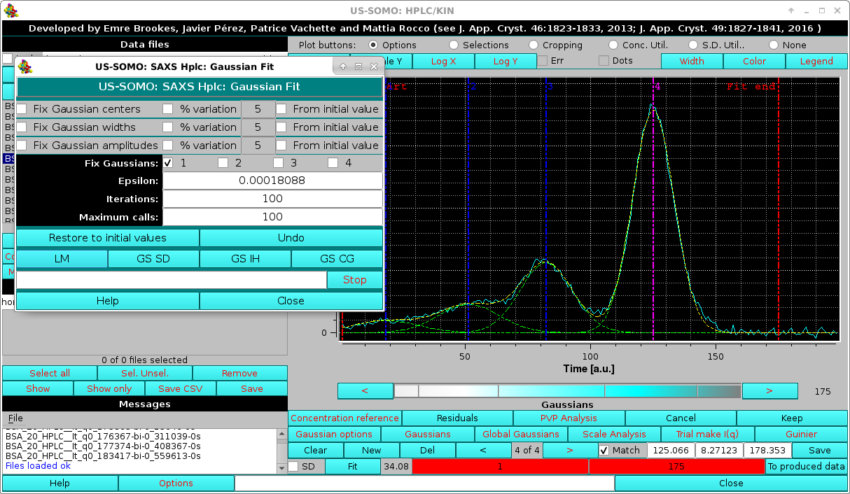 |
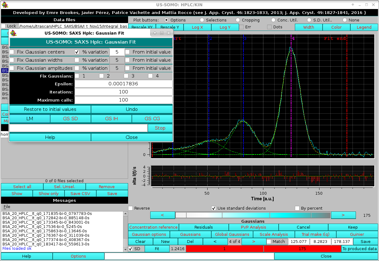
A final round of fitting can then be performed using the SD and allowing a 5% variation on the Gaussian centers at each iteration, until a satisfactory fit of the main peak(s) is obtained:
 |
If some datasets have missing or NaN values for one or more SD values, a pop-up menu will appear listing all the files presenting this problem, and with how many occurrences. The user can then select between three options: drop the datasets containing these non-defined SDs; drop just the frame (or time) point missing the SD(s); or not use SD weighting.
The global improvement of the fit can be also judged by the rmsd (SD checkbox not selected) or χ2 (SD checkbox selected) value which is updated next to the Fit button. The residuals of the fit can be visualized by pressing the Residuals button, which will split the graphics window in two, and show a plot of the fit residuals below the main plot. The residuals plot can be removed by pressing Residuals again (see more below). In the example shown above, the residuals are weighted by the std. dev. associated with the experimental points (SD checkbox selected; a By percent residuals option is also available).
Once a satisfactory fit is reached, pressing Keep will accept the current Gaussians for further work. But to save the parameters of the current Gaussians in a file, the Save button has to be pressed before Keep.
Once an initial set of fitted Gaussians has been produced, it should be globally fitted to all chromatograms. However, performing this operation directly on all chromatograms can be very computationally intensive. For this reason, it is best to perform it on a subset of all chromatograms, and the global fit results are then propagated to all remaining chromatograms. Importantly, in the global fitting procedure the centers and widths of each particular Gaussian are optimized so to be the same across all chromatograms, and only the amplitudes are then fitted.
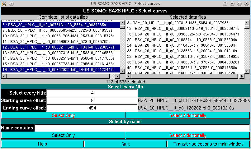
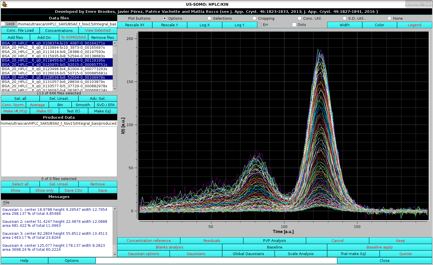
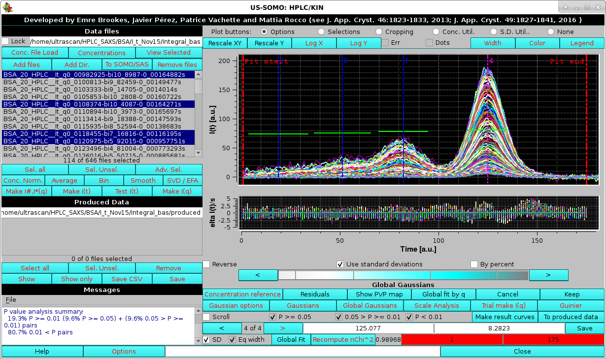
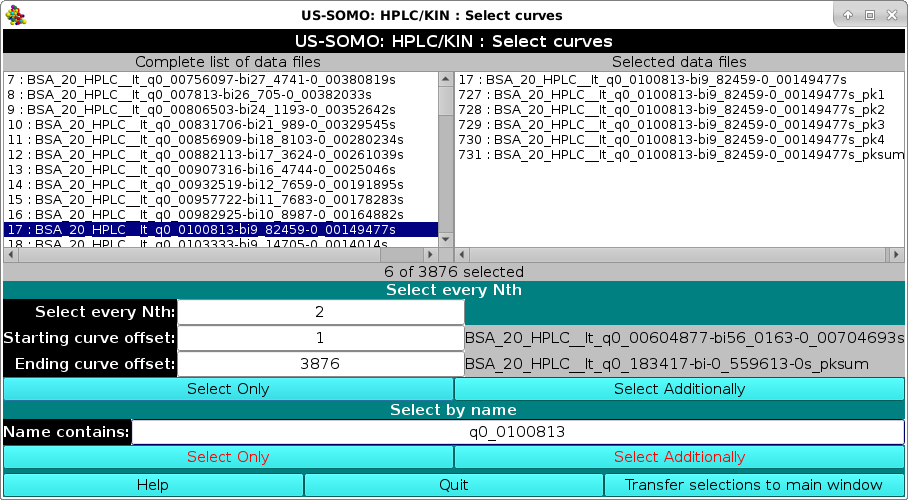
It is advisable to perform the global fitting avoiding the very first few low-q, very noisy, and the last high-q, very low signal I(t) vs. t chromatograms. In the example we are illustrating, we start from chromatogram # 8 (q = 0.007813 Å-1) and select every 4 chromatograms up to # 454 (q = 0.12020 Å-1). The I(t) vs. t chromatogram on which the initial set of Gaussians was optimized is also included (Select Additionally button). Pressing Transfer selection to main window will close the pop-up window and the selected files will be shown in the main HPLC/KIN module graphics window (whose frame for this screenshot has been enlarged so that the information regarding the four Gaussian present in the Messages panel is fully visible):
 |
Turn on is then selected. Global Gaussians will allso restore the saved parameters saved in a file after a satisfactory fitting is attained. For this reason, another pop-up panel will appear:
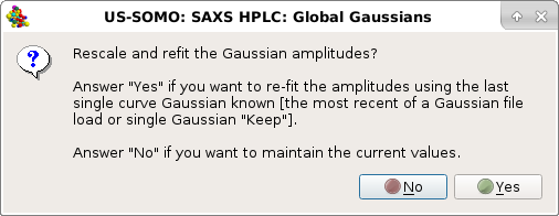
In this case, the answer is Yes, and the amplitudes will be set for all the selected chromatograms.
If datasets having points with missing or NaN std. dev. values are found, a third pop-up panel will appear:
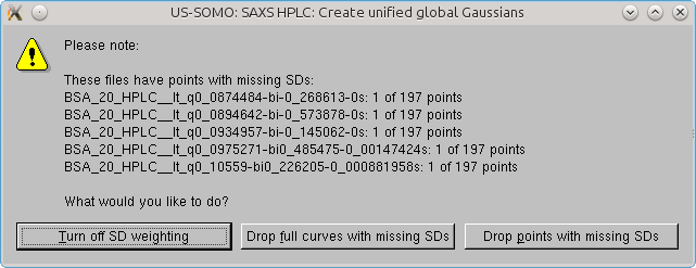
When just a few problematic points are found for each chromatogram, the Drop points with 0 SDs option can be safely used. The global Gaussians operation will then be completed:
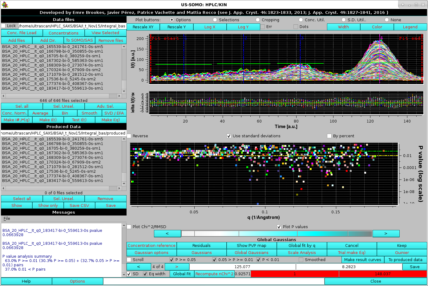
 |
In the image above, the Global Gaussians results on the Nth selected files are shown, together with the grouped fit residuals. The common centers and widhts, not optimized but just based on the initial chromatogram fit, are displayed in the graph as vertical and horizontal bars, respectively. Note that the x-axis scale and the Residuals y-axis scales were manually optimized (right-click on the scale to access the plot options menu). The global P-value analysis for this initial Gaussian propagation is also shown in the Messages panel. Both the residuals and the P-value analysis indicate a poor fitting of the initial Gaussian when just propagated to the other selected chromatograms.
 |
In the image above, the results of the Global fit are shown together with the grouped fit residuals. Furthermore, a new set of tools is available to judge the goodness of the fit.
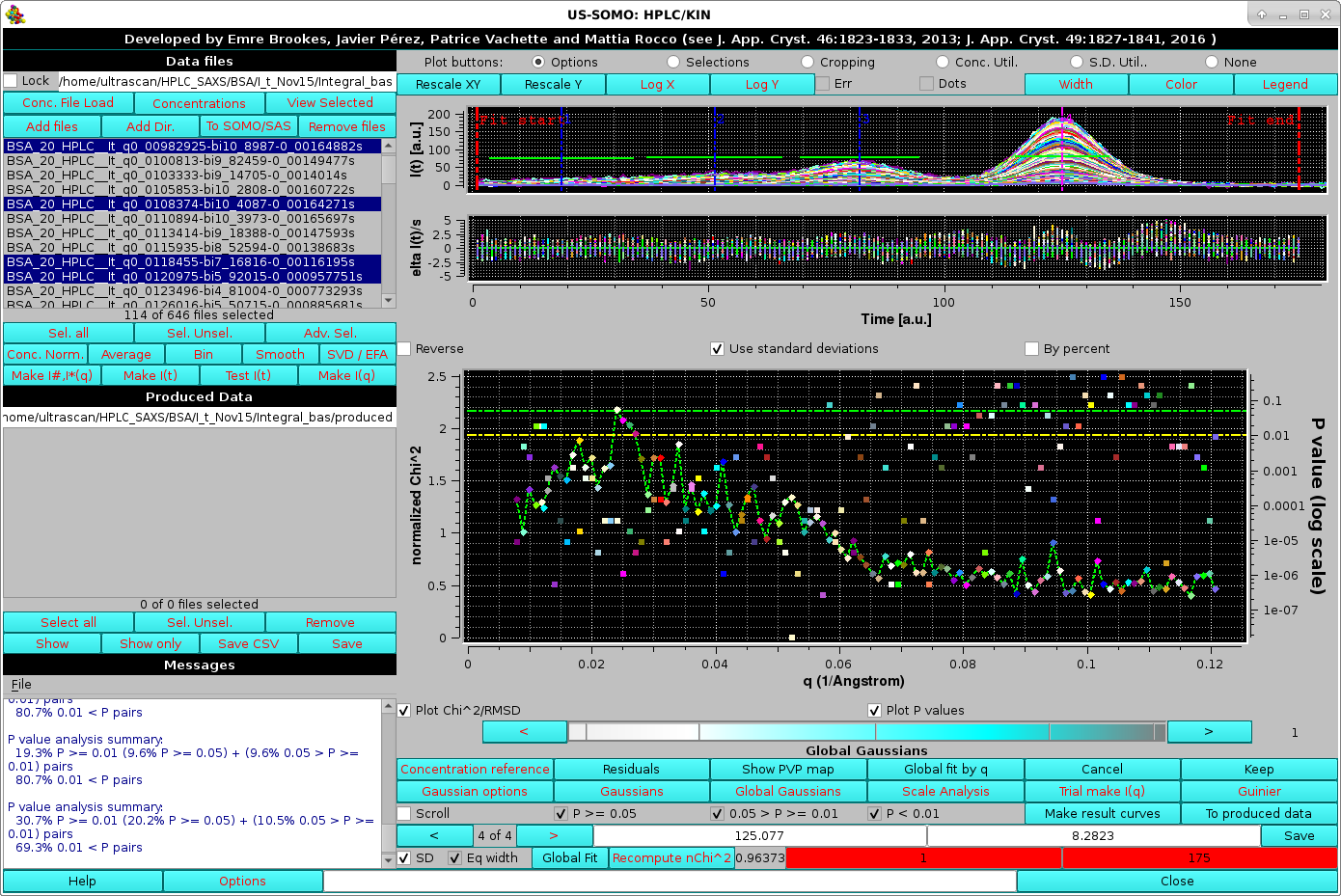 |
In the Global fit by q graph it is possible to visualize either one of or both the two plots, by selecting/deselecting their respective checkboxes positioned just below it (Plot Chi^2/RMSD and Plot P values). The fit is clearly not optimal. Note that in the image above, where both plots are shown, their respective y-axis scales have been manually modified to allow a better visualization of each plot. The dashed green and yellow horizontal lines mark the usual cut-off P-values (P ≥ 0.05, above the green line; 0.05 > P > 0.01 between the green and yellow lines; P < 0.01, below the yellow line).
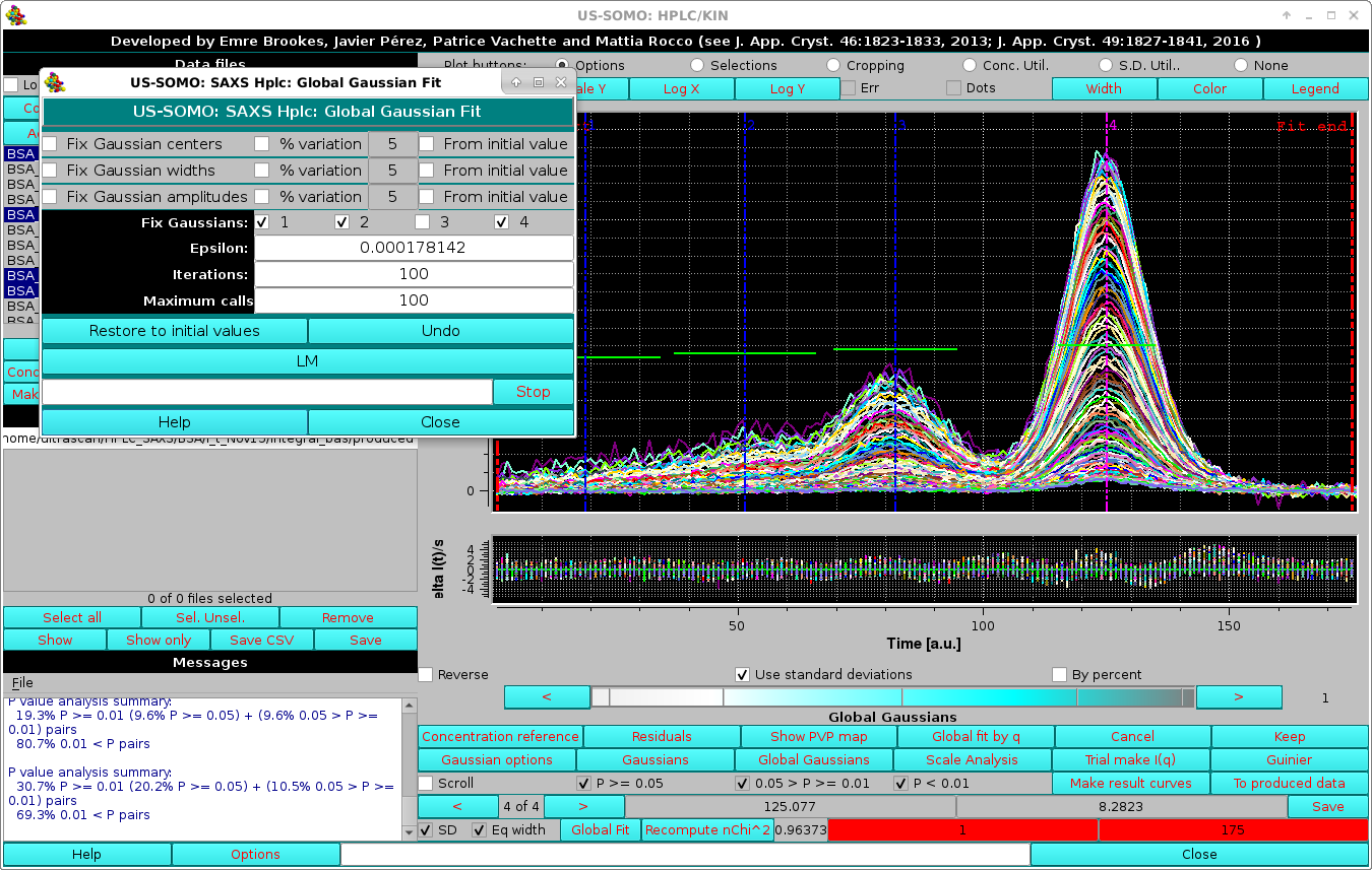
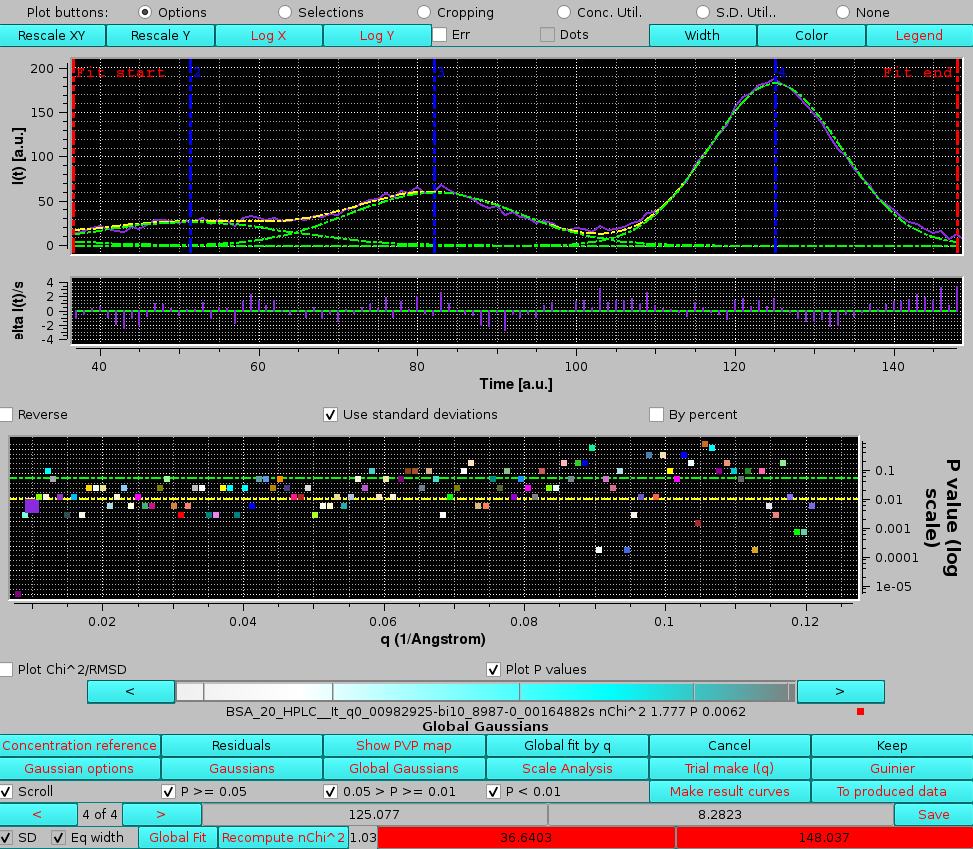
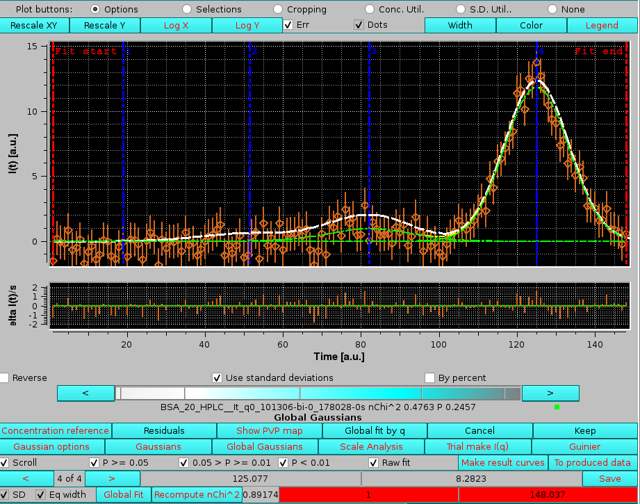
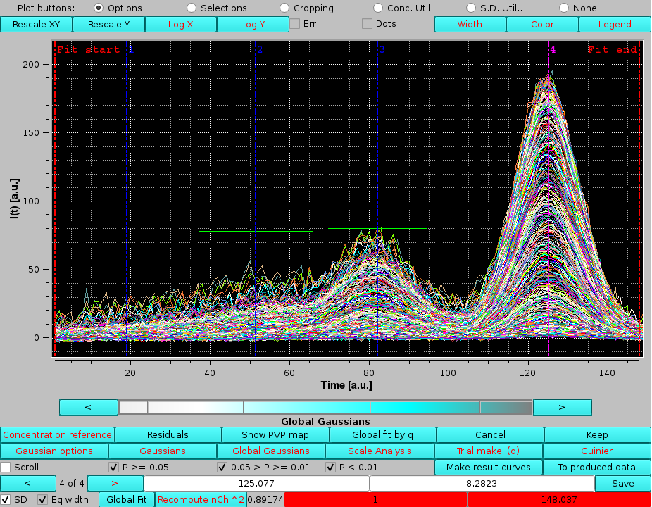
We can move the limits of the fit to exclude the first peak and the tail of the main peak, to concentrate the goodness-of-fit indicators toward the most important part of the fit, including the top (2/3)rds of peaks 2, 3 and 4. Each time the limits are moved, the normalized χ2 and P-values are recomputed by pressing the Recompute nChi^2 button):
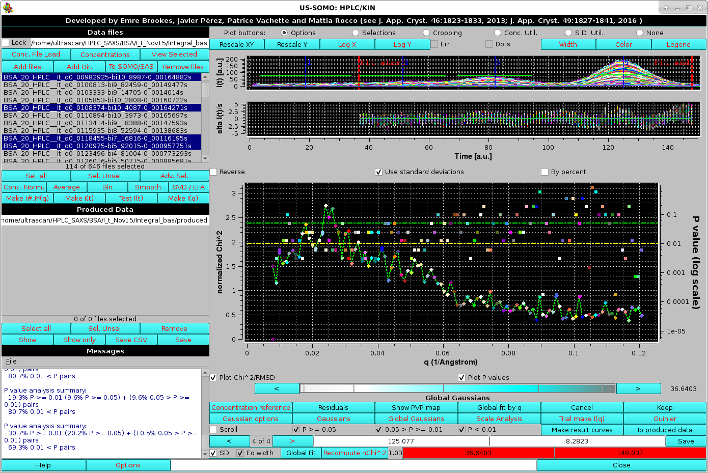 |
With these limits, the normalized χ2 values display "reasonable" values, ≈1.5-2.5 for the lowest q angles (up to q ≈0.035 Å-1), then almost linearly decaying to ≈0.7 for q ≈0.8 Å-1, being stable afterwards, for a global χ2 ≈0.95. Likewise, the P-values show a slight trend toward better values as the q increases, but the distribution of really "bad" P-values appears to be substantially random.
 |
In the image above, only the P-value are shown. The current chromatograms pair is highlighted in the P-values plot by an enlarged symbol (purple square in this case). Scrolling is performed by either using the cyan-scale bar-wheel, or by clicking on the the "<" and ">" buttons placed at its sides. By selecting/deselecting the three checkboxes next to the Scroll checkbox (P >= 0.05, 0.05 > P >= 0.01, P < 0.01), only the subset(s) whose P-values are within those of the selected chechbox(es) will by scrolled.
In the example shown above, by examining the residuals' plot it is clear that the "bad" P-value it is due to a poor fit in the inflection point betweern the 3rd and 4th peaks. If we examine a chromatograms pair just three q values above the first one examined in detail, we can see that oscillations in this zone produce an excellent P-value, although this still appears to be a difficult zone to fit with symmetric Gaussians:
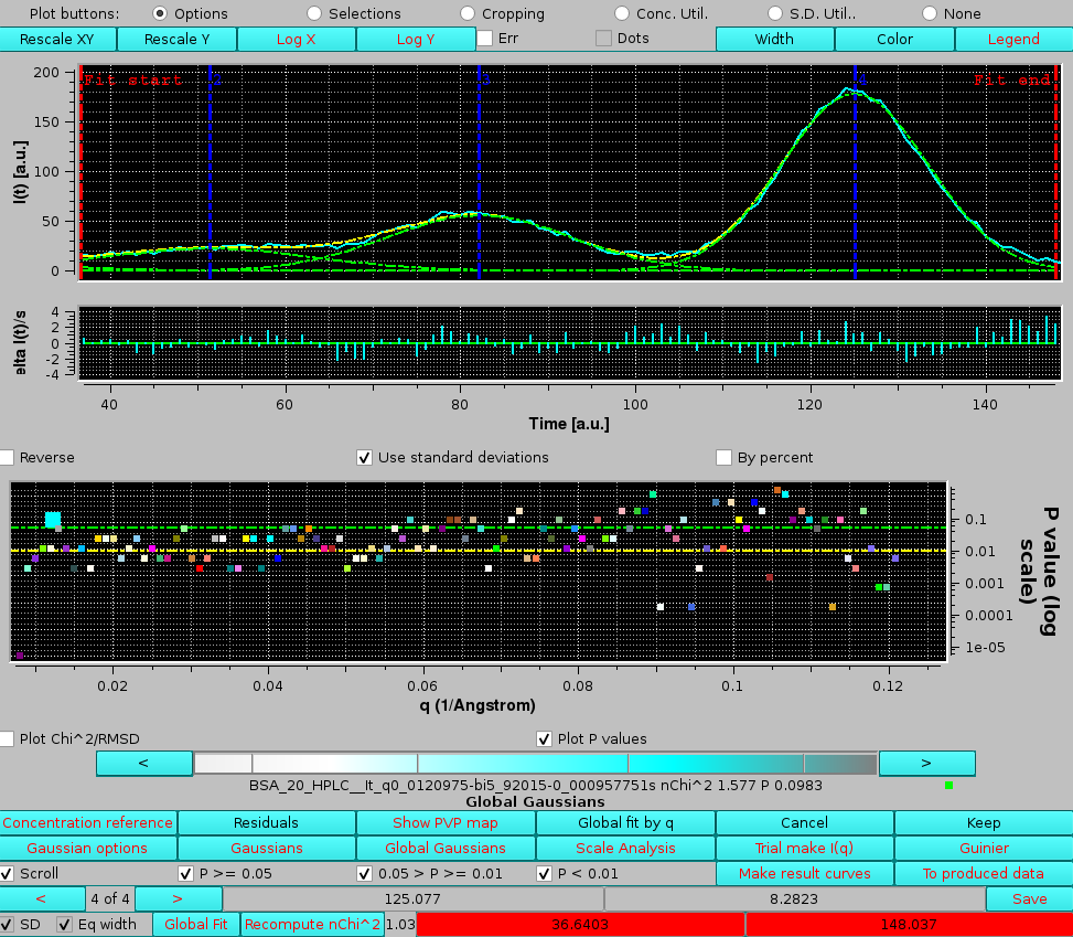 |
The noticeable worse fitting and the end of the main peak could indicate either a slight non-pure Gaussian shape of the peak, or the presence of a small amount of some trailing material in this region.
Also in this case, the answer is Yes, and the amplitudes will be set for all the selected chromatograms.
Again, if datasets having points with missing or NaN std. dev. values are found, a pop-up panel will appear (not shown).
If we hadn't restored the left-side fit limit to include the first peak, another pop-up panel would have appeared:
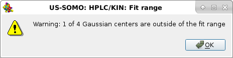
Pressing Ok will allow the operation to complete anyway, and if the results are poor they can be refused by pressing Cancel and proceeding as explained above, leading to a better Gaussians propagation:
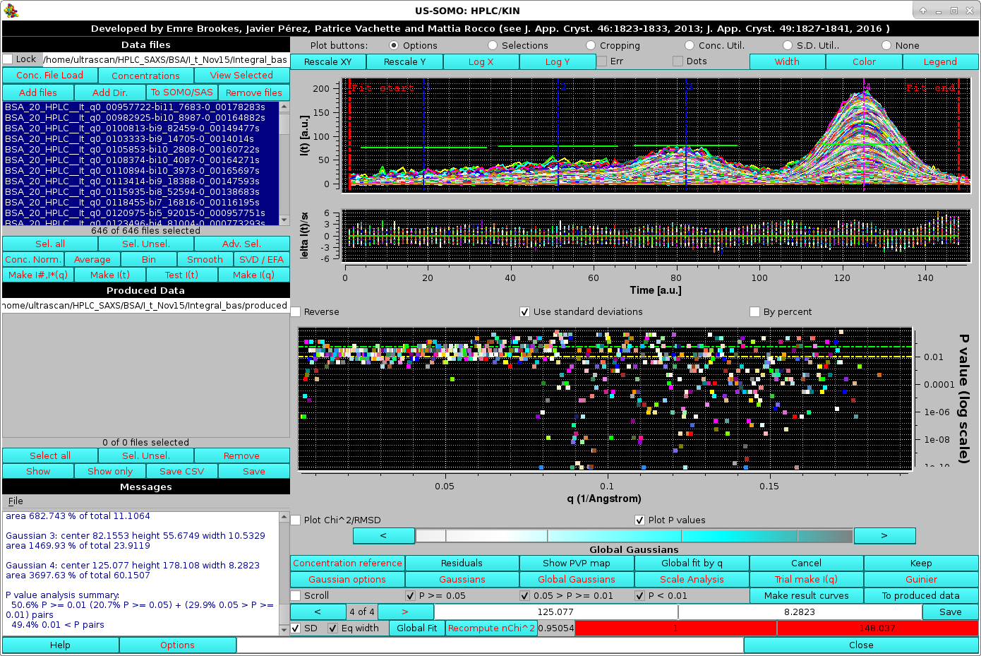 |
The image above shows the global Gaussians results after applying the global fit parameters found on a subset of data to all chromatograms. Save and Keep can then be sequentially pressed to store and accept the global Gaussian results.
Note, however, how the P-values plot shows a large increase of "bad" P-values at increasing q-values. This is due to the global Gaussians propagation failing to reach true mininima by some peaks values getting "trapped" by spikes in the data. To alleviate this problem, starting from the July 2024 intermediate release we offer two alternative ways leading to a better global Gaussians propagation. In the HPLC/KIN Options module there are two checkboxes labeled "Experimental: Global Gaussian Initialization smoothing. Maximum smoothing points:" followed by a field that becomes available if this checkbox is selected, and Experimental: Global Gaussian cyclic fit.
The first feature deals with the problem of how to avoid local minimima when propagating a set of Gaussians optimized on a few chromatograms to all other chromatograms, by resorting to smoothing the data. Especially for high scattering angles, very noisy data, local spikes can lead the optimization of the individual fits to stop before reaching a true global minimum. Smoothing at the fit level alleviates this problem. (Note: importantly, the final decomposition when regenerating the I(q) vs. q data for each peak is done on the original, not on the smoothed I(t) vs. t chromatograms!).
After selecting this checkbox with 7 as the maximum smoothing points, we can return to the HPLC/KIN module and restart Global Gaussians. The pop-up asking for re-fitting the Gaussians amplitudes or keeping the actual values will again appear, and we choose Yes, leading to an iterative procedure where for each chromatogram a smoothing pass increasing from 1 to the maximum chosen points (7 in this case) is launched, followed with the amplitudes fitting. The procedure stops at each chromatogram level when a further increase in smoothing doesn't improve the fit, leading to these results:
 |
The final smoothed data for each chromatogram appear in the Data files and Produced Data sections with the extension "sm-x", with "x" the maximum smoothing value reached. The improvement in the fitting can be seen in the Messages section, where the global "good" P-values have increased from ∼50 % to ∼63 %. The Global fit by q plot also shows an improved distribution of the i>P-values. The effect of the smoothing on any chromatogram can be checked by selecting any pair as in this example, where the maximum smoothing points allowed was reached:
 |
Obviously, while this procedure can resolve some of the local minima problems, it cannot cure poor fitting issues.
The second procedure we developed can be run by choosing the Experimental: Global Gaussian cyclic fit in the HPLC/KIN Options module. If this checkbox is selected, during the initial Global Gaussian fitting instead of directly fitting the all Gaussian curves simultaneously, each Gaussian first is fit sequentially, keeping the others fixed, followed by fitting all Gaussians simultaneously.
After selecting this checkbox, to allow a direct comparison of this cyclic procedure versus the "standard" procedure, the Experimental: Global Gaussian - Enable legacy Gaussian fit display is also checked. We can now return to the HPLC/KIN module and restart Global Gaussians. The pop-up asking for re-fitting the Gaussians amplitudes or keeping the actual values will again appear, and we choose Yes, leading to the cyclic fit being launched (as reported in the Messages section) with these results:
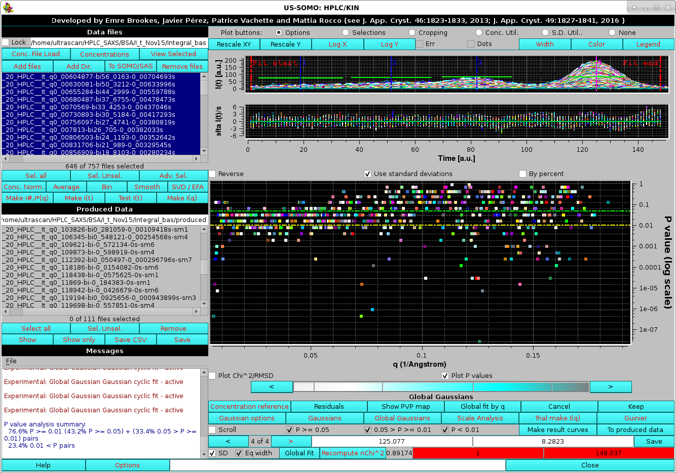 |
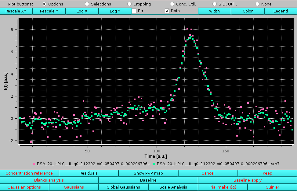
The improvement in the fitting can be seen in the Messages section, where the global "good" P-values have now increased from ∼50 % to ∼76 %. The Global fit by q plot also shows an improved distribution of the P-values. As for the smoothing procedure while the cyclic fit procedure can significantly resolve some of the local minima problems, it cannot cure poor fitting issues. Selecting then the Scroll and the "Raw" checkboxes, we can directly see the effect of the cyclic procedure on any chromatogram, as in this example:
 |
where the sum of the cyclic fit and that of the "raw" fit derived Gaussians are the green and white lines, respectively. The improvement is clear by examining peaks #2, #3, and the main peak (#4): peak #2 has practically some random noise at this high q value, which was still interpreted as a Gaussian in the "raw" fit while the cyclic fit correctly interpreted the signal. For peak #3, the fit is significatly improved, avoiding being caught on some spikes, and even for peak #4 the top appears to be better interpreted.
After exiting from the Scroll mode, Keep can then be pressed to accept these Global Gaussian results for further analysis.
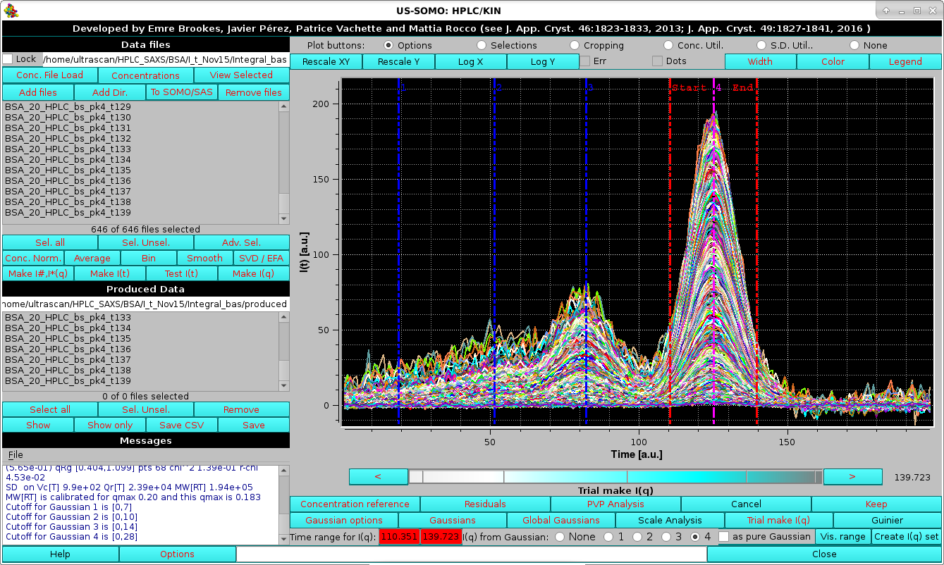
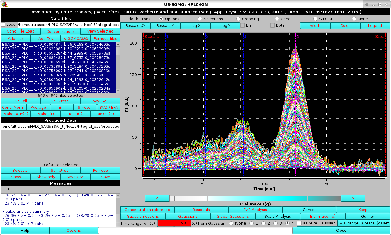 |
The Time range for I(q): two red fields allow selecting a particular region of the chromatograms, by either clicking on each one and then typing in the times, or using the cyan-scale bar-wheel and/or the "<" and ">" buttons placed at its sides. The I(q) from Gaussian: round checkboxes labeled none, 1, 2, 3, and 4 allow selecting which Gaussian will be used to produce the corresponding decomposed I(q) vs. q data, as a pointwise % of the original I(t) vs. t data based on the relative contribution of all Gaussians at that particular point in t space. The square as pure Gaussian checkbox appears once a Gaussian is selected; if it is checked, the actual Gaussian value will instead be used (effectively smoothing the data).
In the first example shown below, we start by first selecting the region of the main peak and checking the 4th Gaussian.
![SOMO HPLC-SAXS Trial I(q) Guinier ME[RT] limit warning pop-up](somo-HPLC-SAXS_MWRT_limit_warning.png)
Pressing Ok will allow access to the new screen:
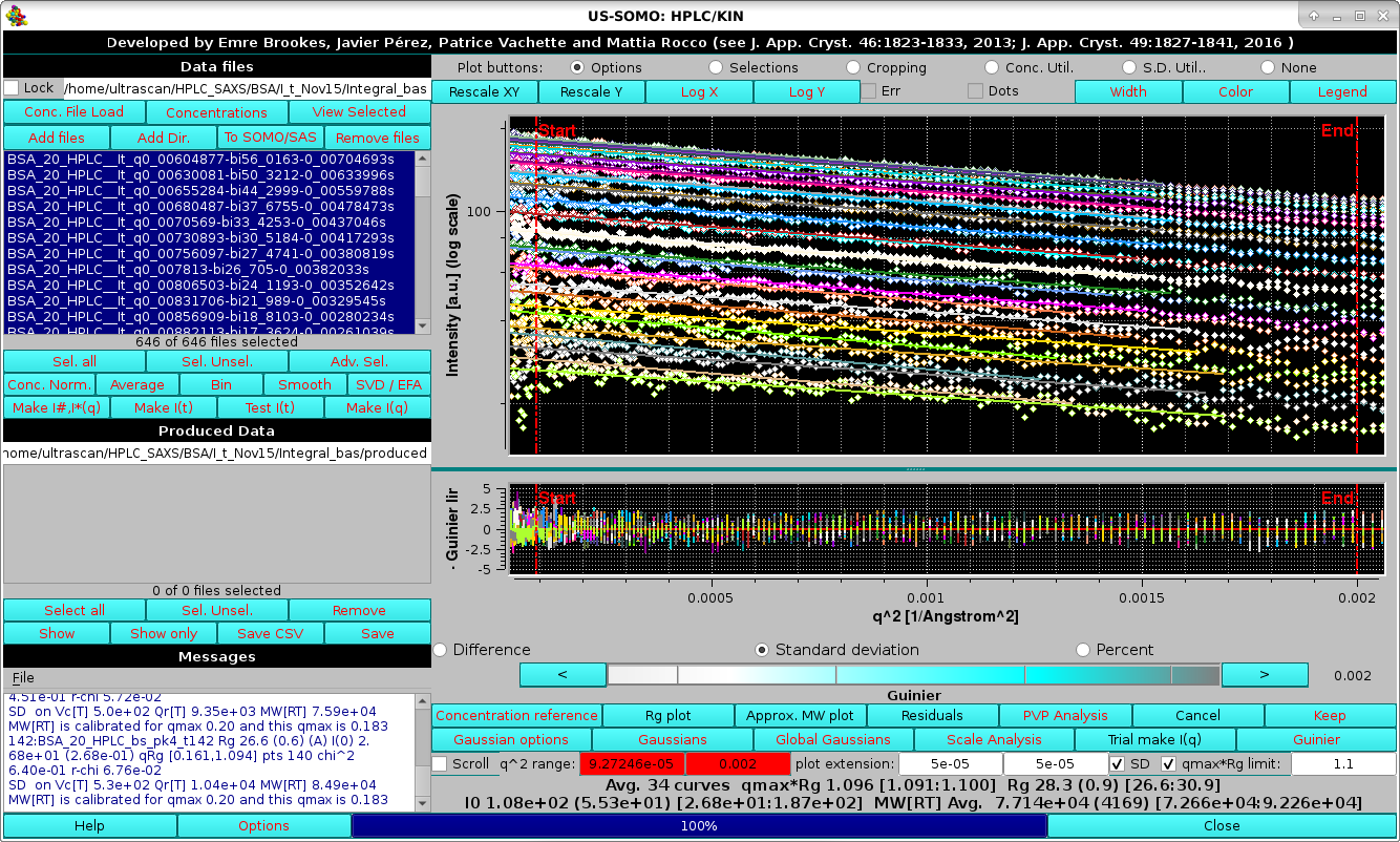 |
where the preset limit for qmax*Rg=1.3 was used. The results of the Guinier analyses and of the MW[RT] calculations for each individual I(q) vs. q curve are reported in the Messages area, while the average values for the entire dataset are reported at the bottom of the command buttons, which now present several new buttons, checkboxes, and fields.
 |
In the image above, the Residuals button was also pressed, with the Standard deviation checkbox selected, allowing to evaluate the cumulative quality of the Guinier analyses.
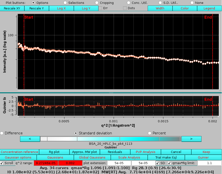 |
scrolling is accomplished by using the cyan-scale bar-wheel and/or the "<" and ">" buttons placed at its sides. Pressing again Residuals will make that plot disappear.
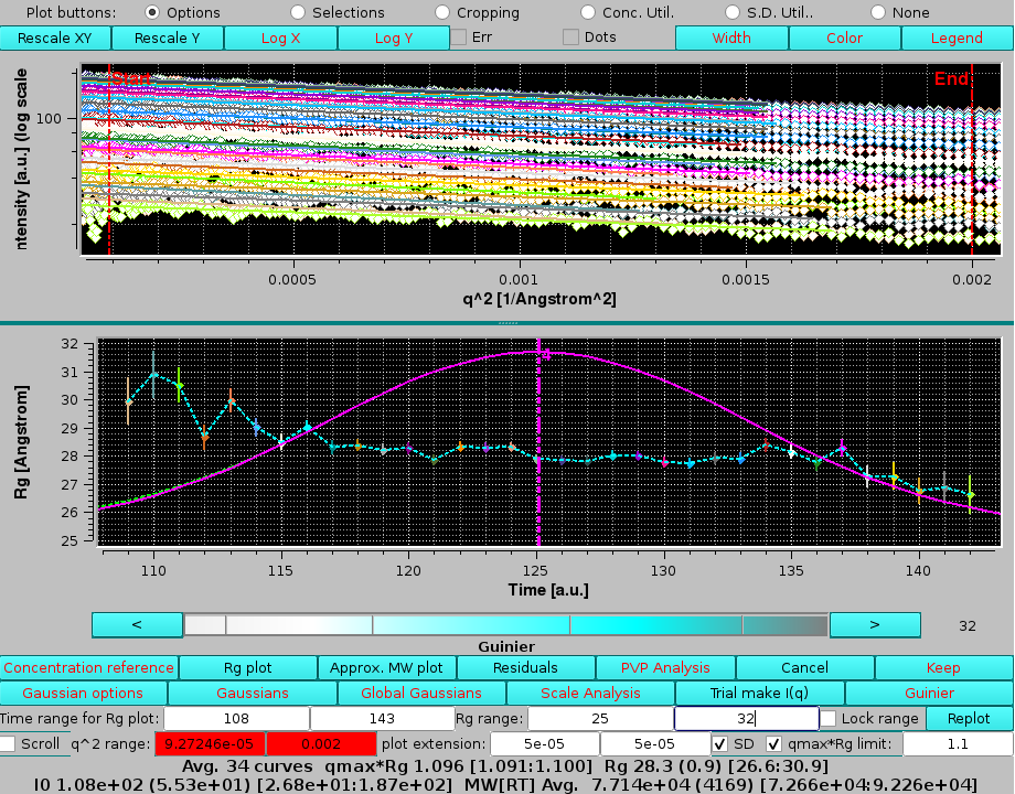 |
The original contribution of the 3rd Gaussian under the main peak can be now evaluated by first clicking on Trial make I(q) and then selecting the I(q) from Gaussian: "none" round checkbox, followed by pressing Guinier and Rg plot:
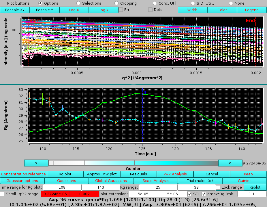 |
here the qmin and qmax limits were also manually reset to the ones used in the previous analysis. As can be seen, there was a slight contribution of the 3rd peak, consistent with near baseline-separation between the 3rd and 4th peaks.
If we perform this analysis selecting the top region of the dimer (3rd) peak (frames 71-91) and its Gaussian, we find very different Rg values, ≈ 43 Å, almost evenly distributed across the peak:
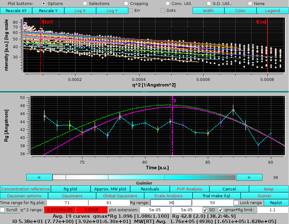 |
here the qmax limits was manually reset. Note that some of the curves present an upward curvature at low q-values, likely indicating a non-ideal baseline correction for this sample.
Finally, the contribution of the 2nd peak under the 3rd peak in absence of Gaussian decomposition can be seen again by selecting the I(q) from Gaussian: "none" round checkbox, followed by pressing Guinier and Rg plot:
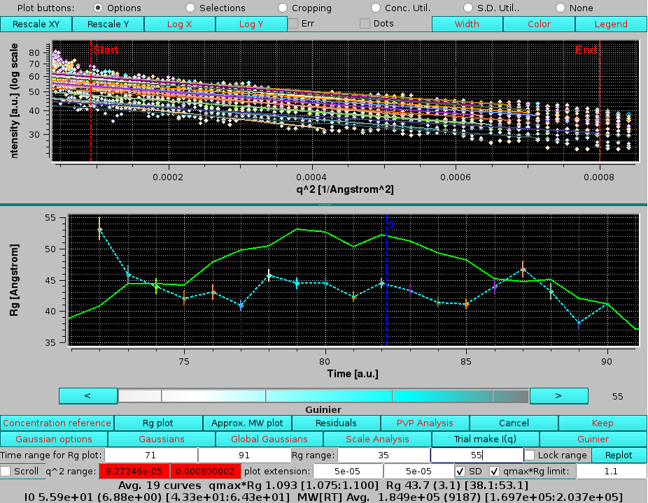 |
finding higher Rg values on the ascending part of the peak, consistent with no baseline separation of these two peaks which was effectively cured by the Gaussian decomposition.
 |
as indicated in the Data files and Produced Data sections, with additional parameters printed in the Messages section. The produced I(q) vs. q curves can be visualized in the graphics window by first exiting from the Trial make I(q) procedure by clicking on Cancel, and then pressing Sel. Unsel. in the Data files section:
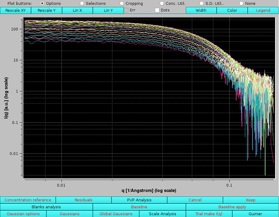 |
here the Log X and Log Y buttons have been pressed to change the x- and -axis visualization mode.
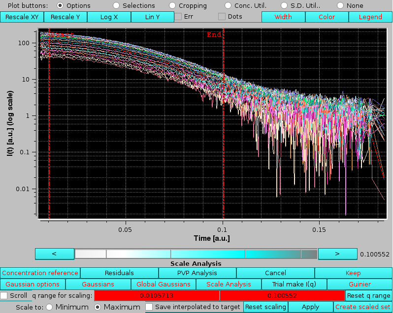 |
here the q limits for the scaling region have been set by clicking on the q range for scaling: red fields and using the cyan-shades bar-wheel to postion the two vertical red lines (pressing the Reset q range button will restore the full q-range).
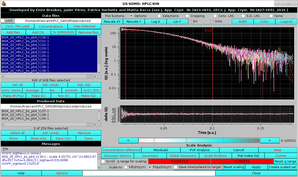 |
with the scaling parameters reported in the Messages section. Here the Residuals button was also pressed.
since we do not need to re-fit the data:
 |
Each individual Gaussian is defined by three to five numbers: the amplitude, width and center, and optionally the distorsions parameters. As such, they are not "curves" in the sense of the loaded files, which are collections of data points. Therefore, the Gaussians can not be visualized with the facilities of the program outside of Gaussian or Global Gaussian modes.
 |
Here, files having "q0_0100813" in their filename were searched and one original dataset and its derived Gaussians were selected and the transferred to the graphics screen:
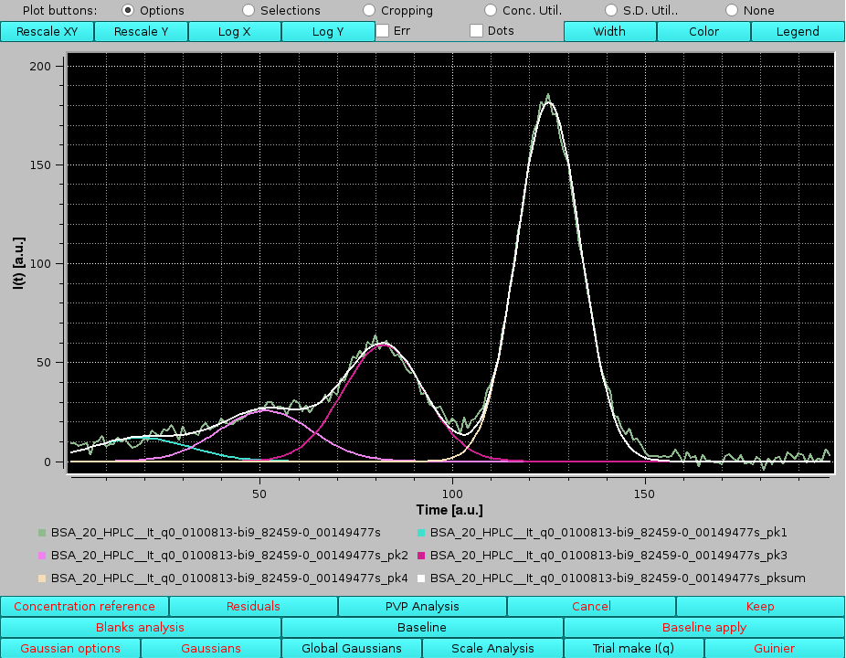 |
To return to the original data, in the Produced Data section we press Select all and then Show only, followed by Sel. Unsel. in the Data files section. Global Gaussians can be again pressed answering No to the pop-up question.
 |
By zooming-in in this graph, any region of the joined original data and their fitting Gaussians can be examined, bearing in mind that the times (or frame numbers) have been sequentially added:
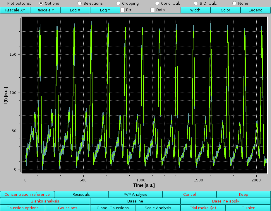 |
 |
The produced data for the individual Gaussians and/or their sum can now be saved or discarded.
 |
the first operation is to rescale it to one of the high intensity but relatively low-noise I(t) vs. t chromatograms. This is done by selecting the two files:
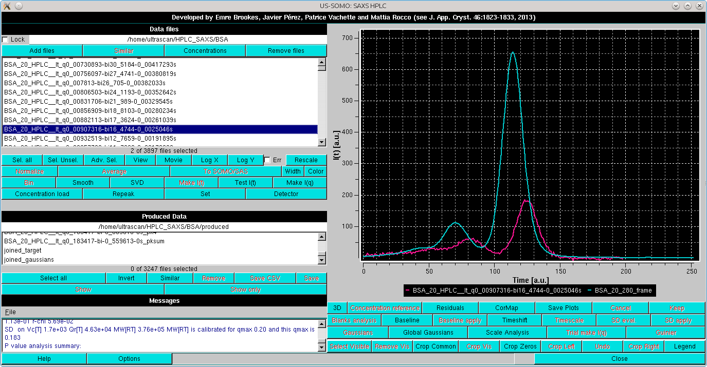 |
and pressing Repeak in the left-side command panel. In case multiple I(t) vs. t were selected, it will bring up a small window asking to identify the target chromatogram:
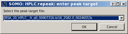
On pressing Ok, a pop-up panel will appear:
 |
Usually the SD are ignored by pressing the first option presented, but the module offers two other alternatives, Match target SD % pointwise and Set S.D.'s to 5% (these two choices could be useful in the Gaussian decomposition procedure if less stringent constraints are sought for the concentration associated data). For this example we choose Match target SD % pointwise. Whatever the choice, the repeak operation affects the data, a new file is generated with "rp" extension and the scaling factor, which will be used to re-generate the proper intensity scale when needed, added at the end of the filename:
 |
At the same time, another pop-up panel will ask if you want to "*Set*" (see below) the repeaked concentration file:
|
If no time-shift between the concentration and the SAXS detectors is present, the repeaked concentration file can then be directly associated with the SAXS datasets. In this case the answer will be No, since the two chromatograms are still time-shifted one in respect to the other.
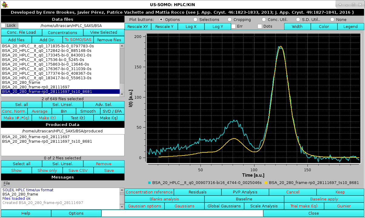
 |
The value of the timeshift is reported in the field next to the cyan-shades bar-wheel.
Cancel will stop the operation.
Keep will keep the time-shifted data. The produced data will have the timeshift value added to its filename on saving.
Then, the pop-up panel will ask if you want to "*Set*" the repeaked concentration file:
|
Answering "yes" will then associate the re-peaked, time-shifted concentration data to the I(t) vs. t SAXS dataset under analysis. This operation can be anyway performed at any time by selecting only a concentration chromatogram dataset, and pressing Set. The concentration chromatogram shown in this example is then cropped to remove the extra frames on the right side, matching the SAXS I(t) vs. t chromatograms:
 |
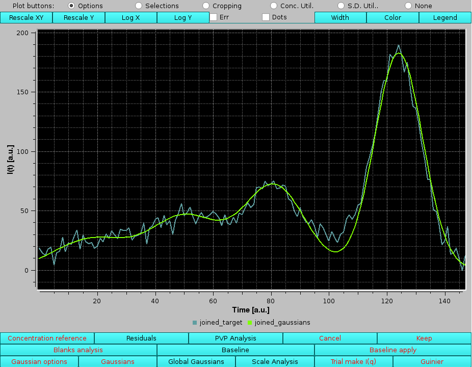
The re-peaked, time-shifted concentration chromatogram can be now fitted with Gaussians, using for initialization the set derived from the I(t) vs. t chromatograms (note: it is mandatory that the same number of Gaussians be used for both the concentration and I(t) vs. t chromatograms).
This is done by first selecting only the concentration chromatogram and then pressing Gaussian, which will bring up the current Gaussian parameters automatically rescaled to the highest intensity in the concentration chromatogram:
 |
Pressing Fit will then bring up the Fit window (see here) and an initial round is done by keeping fixed both the position and widths:
 |
If necessary, a refinement can be done by keeping fixed the smallest, front eluting peak(s), and allowing only a limited shift to a % of the initial values from the widths and positions determined from the SAXS data (suggested: 2-3% max). This should compensate for slight misalignment between the concentration and SAXS detectors chromatograms:
 |
As evidenced in the image above, some band broadening has occurred between the UV-VIS and SAXS detectors. While the issue appears to be relatively minor here, it can be more serious. To at least partially mitigate this issue, we have implemented a re-shaping routine that re-aligns the shape of the concentration detector chromatogram to that of the SAXS detector chromatograms. It is based on determining first the area under each Gaussian peak in the concentration chromatogram after fitting it with the SAXS-derived Gaussians with minimal centers and widths changes, as described above. Then, when the Make I(q) routine is launched, the concentration chromatogram Gaussians can be optionally re-shaped on the SAXS-optimized Gaussians, keeping their areas fixed and adjusting the other parameters (see below).
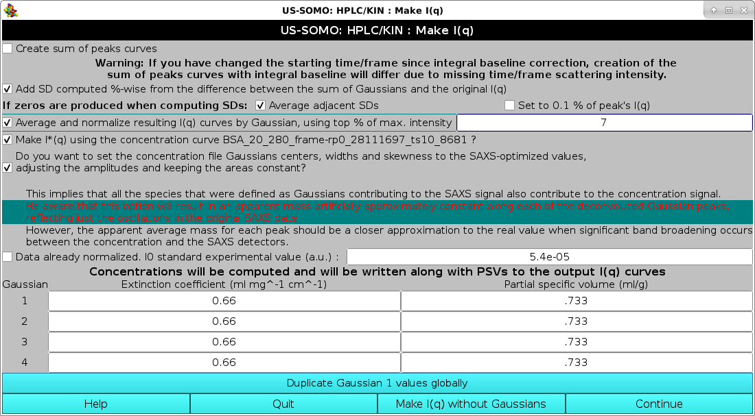 |
A description of this module can be found here.
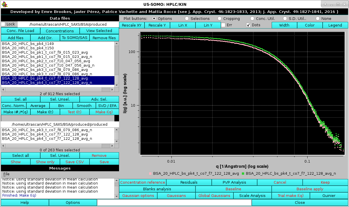
At the end of the Make I(q) operations, if the Average and normalize resulting I(q) curves by Gaussian, using top % of max. intensity" checkbox had been selected, the graphics window will report the averaged curves for each Gaussian-decomposed peak:
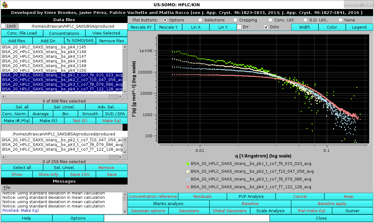 |
shown here in log10-log10 mode and after zooming. Note that since the Make I*(q) using the concentration curve "filename"? checkbox was also selected, we have produced I*(q) vs. q data in [g/mol] units. The intercepts at q=0 then give an approximate molecular weight estimation. This could be immediately verified by selecting a single averaged I*(q) vs. q dataset, like peak #4, and pressing the Guinier button:
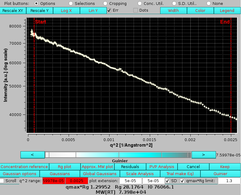 |
Here we can see that the Guinier-extrapolated I*(0) gives a value that although a bit high is consistent with monomeric BSA (∼66,500 g/mol). The Rg value is in excellent agreement with that computed from the structure (28.3 Å).
If the Make I*(q) using the concentration curve "filename"? checkbox is not selected, two averaged I(q) vs. q curves for each Gaussian-decomposed peak will be produced, simple average and average normalized by the concentration:
 |
Here we see just the two I(q) vs. q curves for peak #4.
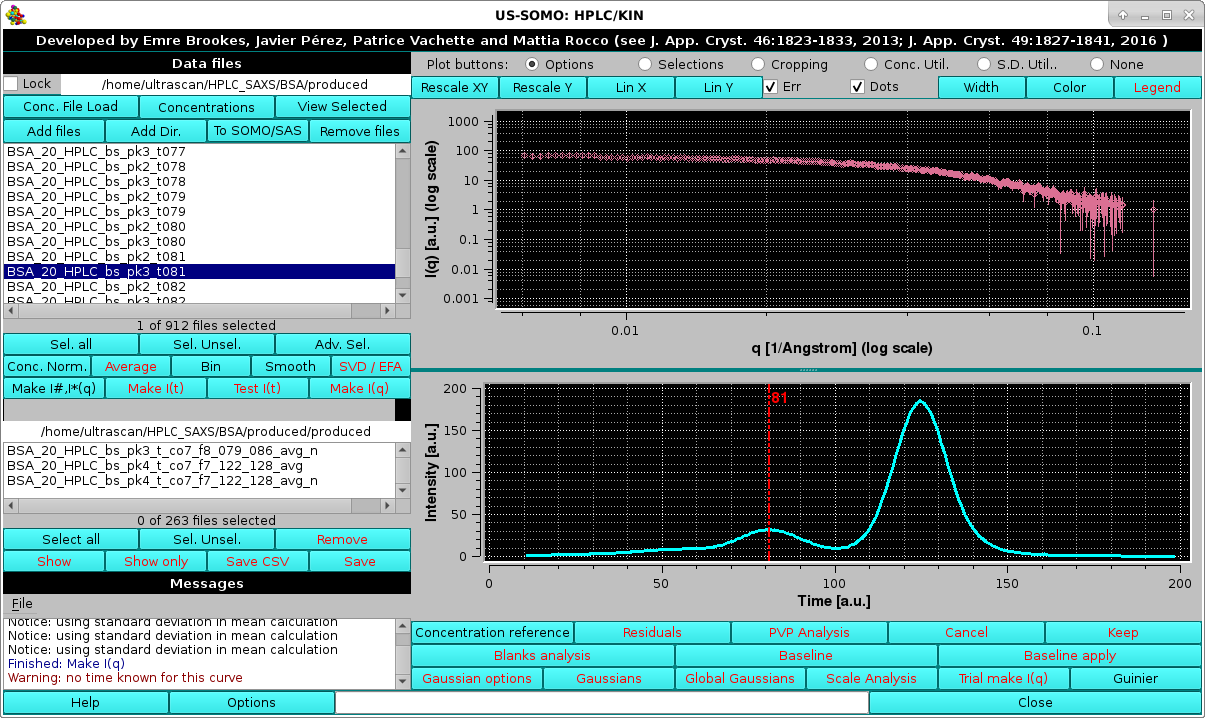 |
In the example shown above, the I(q) vs. q data for the decomposed peak #3 frame #80 are shown with their associated errors, and below it the position of this dataset is shown by the vertical red line on the associated concentration cromatogram. Each time a different chromatogram is selected, its position will be mapped on the concentration plot.
Pressing the Concentration reference button again will make this additional plot disappear.
Finally, the data shown in any of the plots currently visualized can be saved in csv-formatted files by pressing the Save plots button accessible from the Selections checkbox at the top of the graphics window. This will open a pop-up dialogue window where the location and the root filename for the cvs files can be set.
This document is part of the UltraScan Software Documentation
distribution.
Copyright © notice.
The latest version of this document can always be found at:
Last modified on July 11, 2024.