
| |
Manual |
The full screen images showing the US-SOMO: SAS Functions module have NOT been updated to reflect the additional buttons for the new functions available from the July 2024 release, as they not affect the detailed description of the IFT module as originally reported (see below).
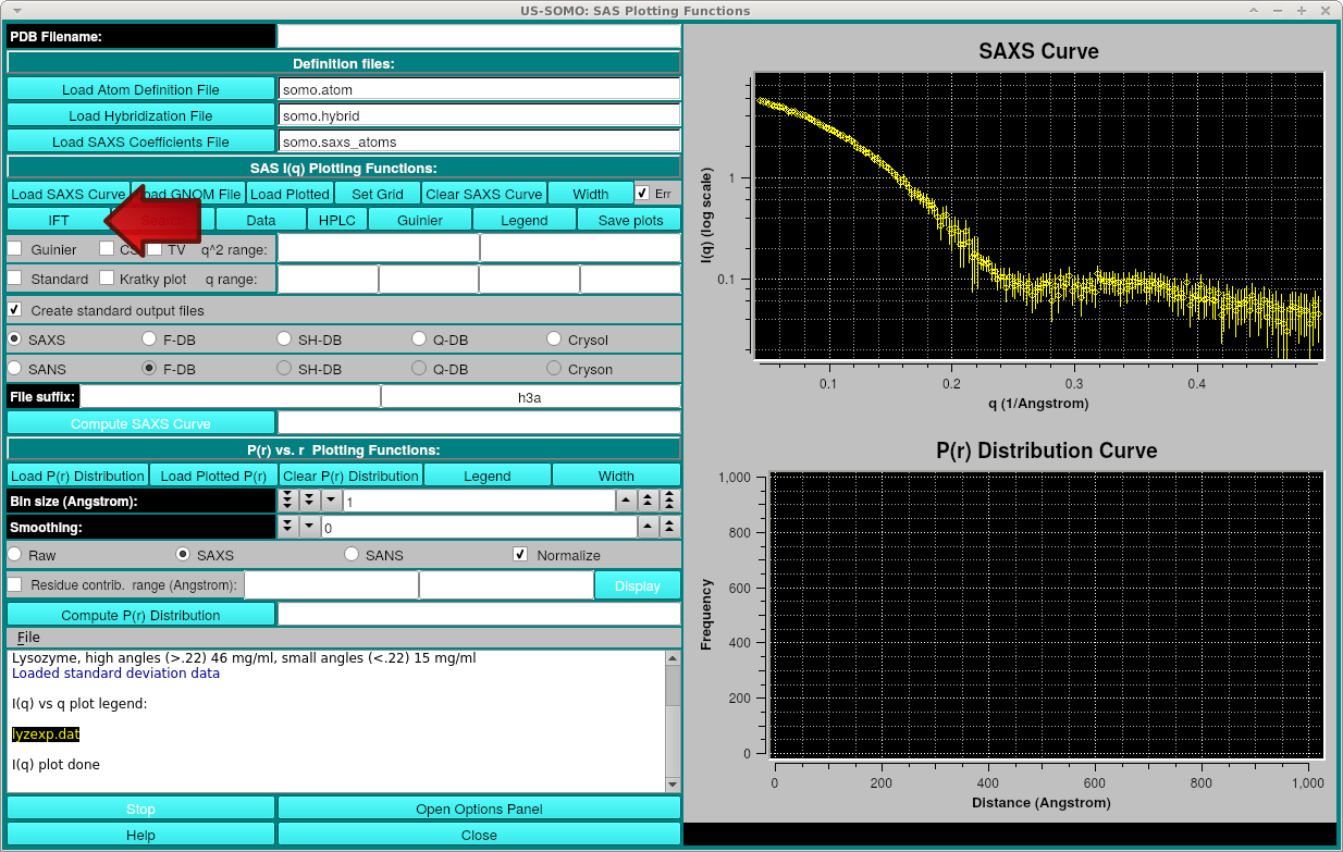
The IFT module can be run by simply pressing the IFT button after loading an experimental SAXS curve into the SOMO-SAS Simulation module.
Note that this method requires that the SAS curve contains a full set of experimental errors. If none are loaded, a messagebox will appear stating this.
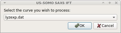
If you have multiple SAS curves loaded with experimental errors, a window will appear asking you to choose which one to process:
However, starting from the July 2022 intermediate release, it is now possible to sequentially process multiple I(q) datasets with the IFT method, utilizing the SOMO SAXS/SANS Load, manage, and process SAS data module.
After pressing the IFT button, the IFT window will appear:
The Indirect Fourier Transform (IFT) Module transforms experimental I(q) curves to produce the pairwise distance distribution histogram P(r) curve using Bayesian Analysis.
This module is an interface to BayesApp of Steen Hansen (J. Appl. Cryst. (2000). 33, 1415-1421;
J. Appl. Cryst. (2008) 41, 436-445;
J. Appl. Cryst. (2012). 45, 566-567;
J. Appl. Cryst. (2014). 47, 1469-1471)
The method of Glatter (Glatter, O. (1977). J. Appl. Cryst. 10), requires prior estimates of Dmax and a regularization parameter. Hansen introduced methods to
determine these parameters automatically using Bayesian Analysis methods.
Further details about the program can be found in the above references.
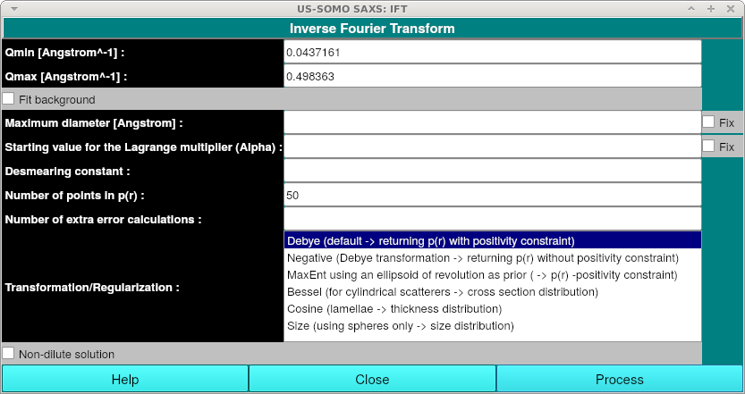
No data entry is required. You can simply press the "Process" button to begin the IFT run. Alternatively, you can specify any or all of the following information:
Qmin [Angstron^-1]:Optionally specifiy the minimum q value to be used. Note that the field is populated by the minimum q value from the experimental data curve.
Qmax [Angstron^-1]:Optionally specifiy the maximum q value to be used. Note that the field is populated by the maximum q value from the experimental data curve.
Fit background If checked, a constant (flat) background will be fitted to the data. Not generally recommended, as your data should have already been properly buffer subtracted.
Maximum diameter [Angstrom]: Optionally enter starting value for the maximum diameter of the scatterer in Angstroms.
Fix (Maximum diameter): Fix the defined maximum diameter. This will override the Bayesian prior distribution for the maximum diameter. Not recommended unless you are very sure.
Starting value for the Lagrange multiplier (Alpha): Optionally enter the starting value for the logarithm of the Lagrange multiplier (usually between -10 and 20). Larger values will give smoother distributions or - for the MaxEnt (see Transformation/Regularization below) constraint: an estimate which is closer to the prior ellipsoid of revolution.
Fix (Lagrange multiplier): Fix the Lagrange multiplier. This will override the Bayesian prior distribution for the Lagrange multiplier. Not recommended unless you are very sure.
Desmearing constant: Optionally enter a correction for slit smearing. Default is no smearing. Enter value for constant c as given by the expression: I_smear(q) = integrate P(t)*I(sqrt(q**2 + t**2)) dt with the primary beam length profile: P(t) = c/sqrt(pi) * exp(-c**2*t**2).
Number of points in p(r): Optionally enter the number of points in the estimated function p(r): more points increase the cpu-time. Default: 50, Maximum 100. If you do not specify also a Maximum diameter, this tends to simply increase the tail of the P(r) distribution.
Number of extra error calculations: Optionally Input number of extra error calculations (maximum 1000). Entering a large number will improve the error estimate, but require more cpu time. In some cases it may be a little tricky to obtain a decent error estimate. Try testing a couple of values to see the effect.
Transformation/Regularization: This option lets you select from multiple transformation and regularization methods:
N.B. The Bessel, Cosine and Size options do not produce a P(r) curve, but rather produce histographic representations of cross section, thickness and size distributions respectively.
Non-dilute solution: Check for non-dilute solutions. Additional fields will be shown when this is checked:
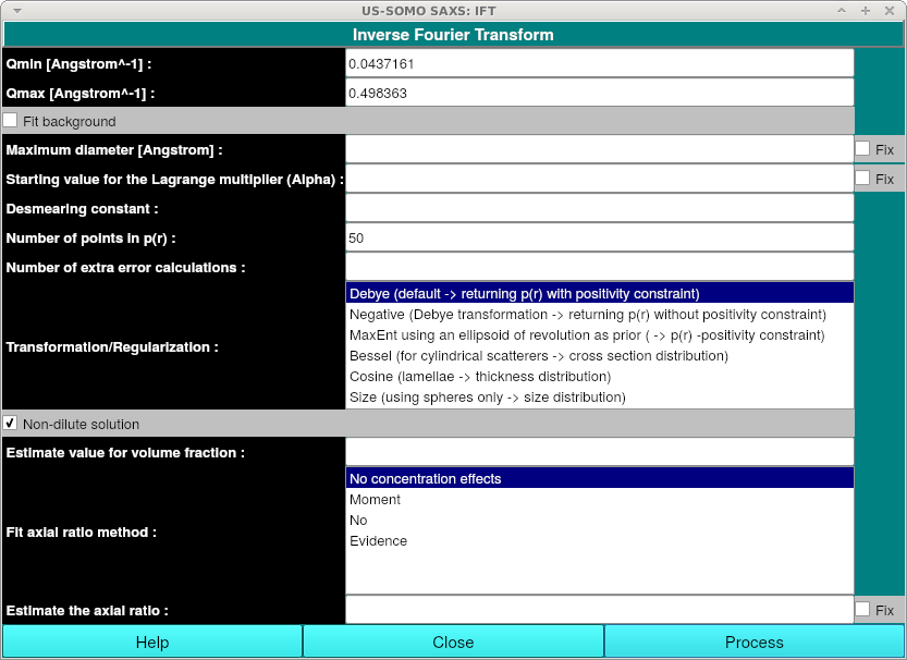
Estimate value for volume fraction: Optionally enter the value for the volume fraction. The exact value entered here may influence the result when the information content of the data is low. Start with a small number e.g. 0.01 to avoid numerical instabilities and long cpu times.
Fit axial ratio method: Optionally enter the method for fitting the axial ratio.
Estimate the axial ratio: Optionally enter an estimate of the axial ratio.
Fix (Estimate the axial ratio): Fix the estimated axial ratio
The following buttons are available at the bottom of the window:
Help Brings up this help page in a web browser.
Close Closes the window. No processing will be done.
Process Process the IFT.
After pressing Process, the progress will be displayed in the text area:
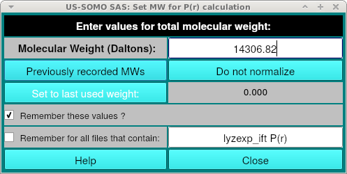
Where you can enter the molecular weight. This is used for scaling of the P(r) curve and if you do not have a molecular weight, you can click "Do not normalize". If you have previously loaded a PDB into the main SOMO window during the session, or entered a molecular weight for a differently named curve, you can select it from "Previously recorded MWs".
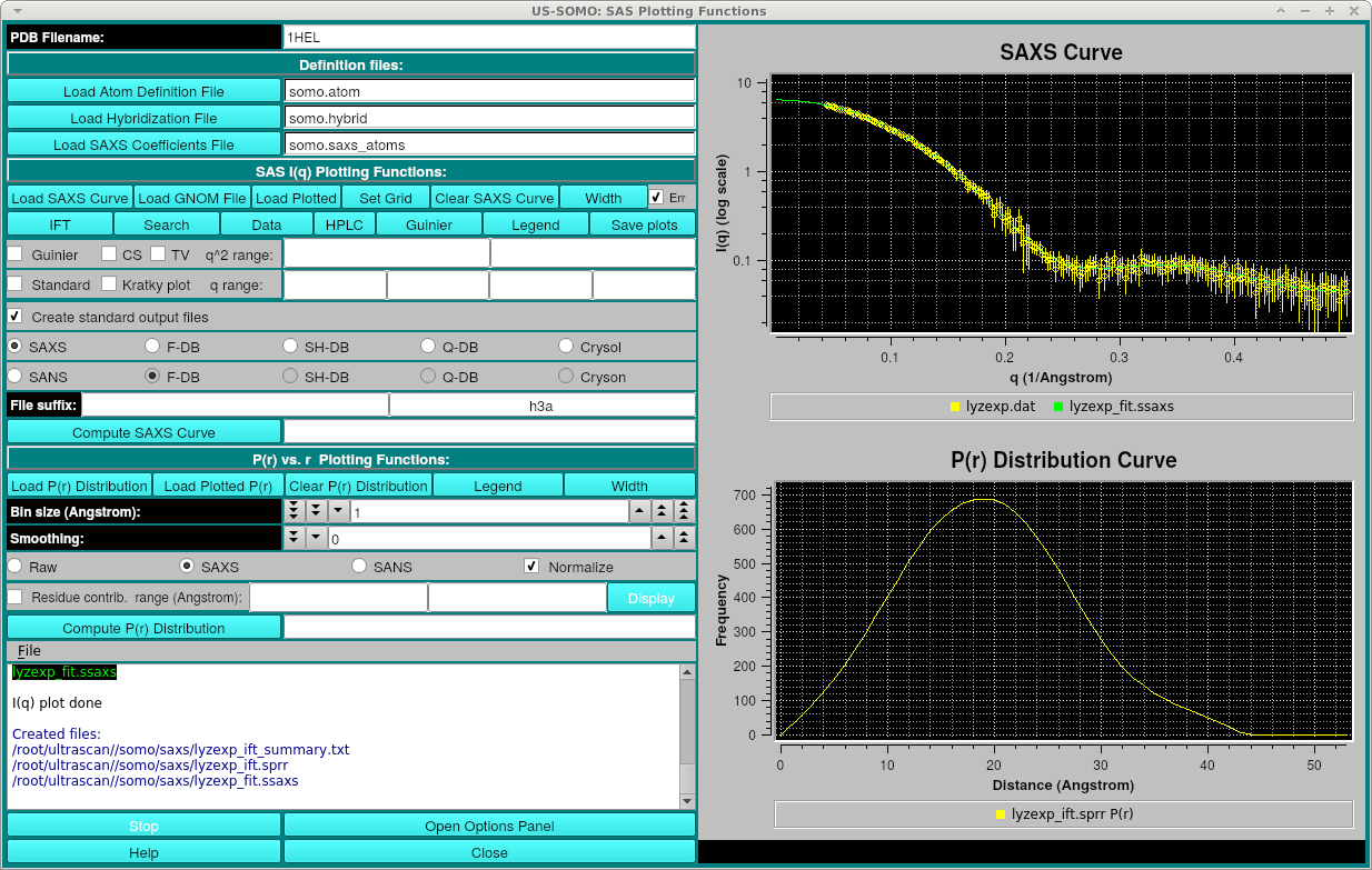
After processing, the three files created are: the original_file_name_summary.txt containing the summary information including Rg, axial ratio, chi^2 and Dmax, original_file_name_ift.sprr containing the P(r) final curve data and the original_file_name_fit.ssaxs file which is the smoothed I(q) curve back-computed from the P(r). The P(r) and smoothed I(q) curves will be displayed, for example (with Legends and error bars on):
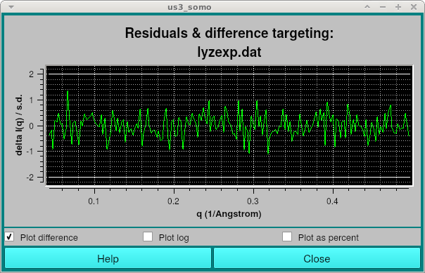
Additionally, a window showing the residuals between the smoothed I(q) curve and the experimental data will be shown:
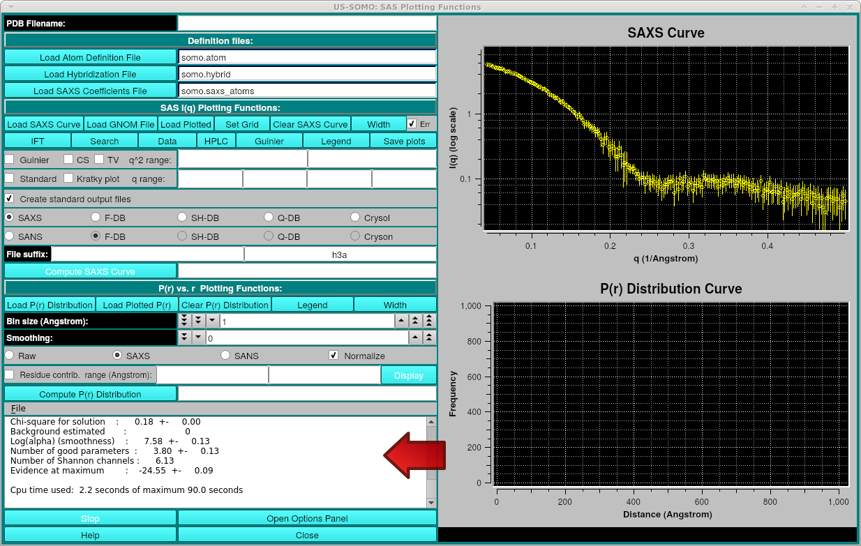
Looking more closely at the output:
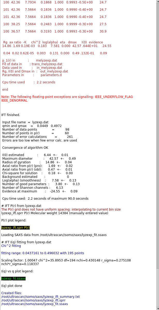
The dark red text is from the direct output of the program. Details of the progress are written during the run, including values of some parameters and the chi-square fit of the back-generated I(q) to the experimental data. There occasionally may be IEEE errors in red, this is generally ok and typically happens for values of parameters that produce bad solutions during the search. After "IFT finished" in black, appear the summary data, including a note about "Convergence of algorithm":
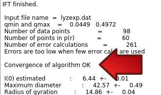
It should read "OK" or at least "almost OK". If it is "NOT OK", then you could try fewer Number of points p(r) and/or provide estimates of Maximum diameter and/or Starting value for the Lagrange multiplier (Alpha).
Additional information including the values and standard deviations for the parameters follows the "Convergence of algorithm" message.
After summary information, the original_file_name_ift.sprr and original_file_name_fit.ssaxs files are loaded, and the normal details of loading a file are written.
The P(r) produced generally does not have uniform grid spacing, so it will be rebinned for display, but the written file will retain the original r-grid.
Finally, the files created with their full paths are shown. These files are now available for general usage within the SOMO-SAS Simulation module.
This document is part of the UltraScan Software Documentation
distribution.
Copyright © notice.
The latest version of this document can always be found at:
Last modified on June 14, 2024. Description of the IFT module as of June 29, 2022.