Manual

Last updated: December 2017

Synopsis

SEC-SAXS data analysis involves repeated curve comparisons and decisions regarding their similarity. This problem has recently been addressed by Franke et al. (Franke D, Jeffries CM, Svergun DI. Correlation Map, a goodness-of-fit test for one-dimensional X-ray scattering spectra. Nature Methods, 12, 419-422, 2015) in a paper in which the authors propose a novel goodness-of-fit test for assessing differences between one-dimensional datasets using only data point correlations over the recorded q‑range or part of it, independently of error estimates, named Correlation Map (CorMap for short). We implemented a routine derived from the calculations described in Franke et al. (2015), in which we essentially perform pairwise comparison of two scattering patterns. In this case, the probability of similarity between the two curves (two different frames or experimental and calculated intensities) may be quantified by evaluating the probability (P‑value) that the largest observed stretch of constant sign correlations be observed by chance. If the P‑value is less than a given threshold, the two curves can be considered as statistically different. We refer the reader to the original article for more details on the method.

When comparing a set of scattering frames, we perform all pairwise comparisons. We present the results in a synthetic way by plotting a square matrix in which the dot (i,j) contains the respective pairwise P-value represented using a three color code¹: green for P ≥ 0.05, yellow for 0.01 ≤ P < 0.05 and red for P < 0.01, when not using the Holm-Bonferroni adjustment; the same color code is utilized using the adjusted acceptance threshold when applying the HB procedure. This pairwise P‑value map is first analyzed in terms of the distribution of values between the three classes with an emphasis on the % of “red” dots. In our unadjusted comparative approach, this is complemented by an evaluation of the average red cluster size, defined as maximal groupings of horizontally and/or vertically adjacent “red” dots. After careful examination of several indicators derived from the pairwise P-value map analysis, average red cluster size was chosen as the most reliable one to determine the global similarity between all frames of the considered subset. However, we have observed that red P-values are too few for clusters to be present when the Holm-Bonferroni adjustment is applied. In this case, the percentage of red pairs is used as the indicator. When the unadjusted comparative approach is used, conclusions are reached regarding the global similarity within the dataset of interest from the comparison of the resulting distributions obtained for that dataset and for the reference set.

We also provide a q_max cutoff for all P-value comparisons, which is by default 0.05 Å^‑1 but can be changed by the user. The primary purpose of this cutoff is to reduce the number of points compared and to focus the comparison in the region of greatest signal information and thereby increase the sensitivity of the probability test.

Details

We start with an example. Suppose we select two I(q) curves (in this case taken near the peak of an SEC-SAXS Lysozyme dataset) as shown below.

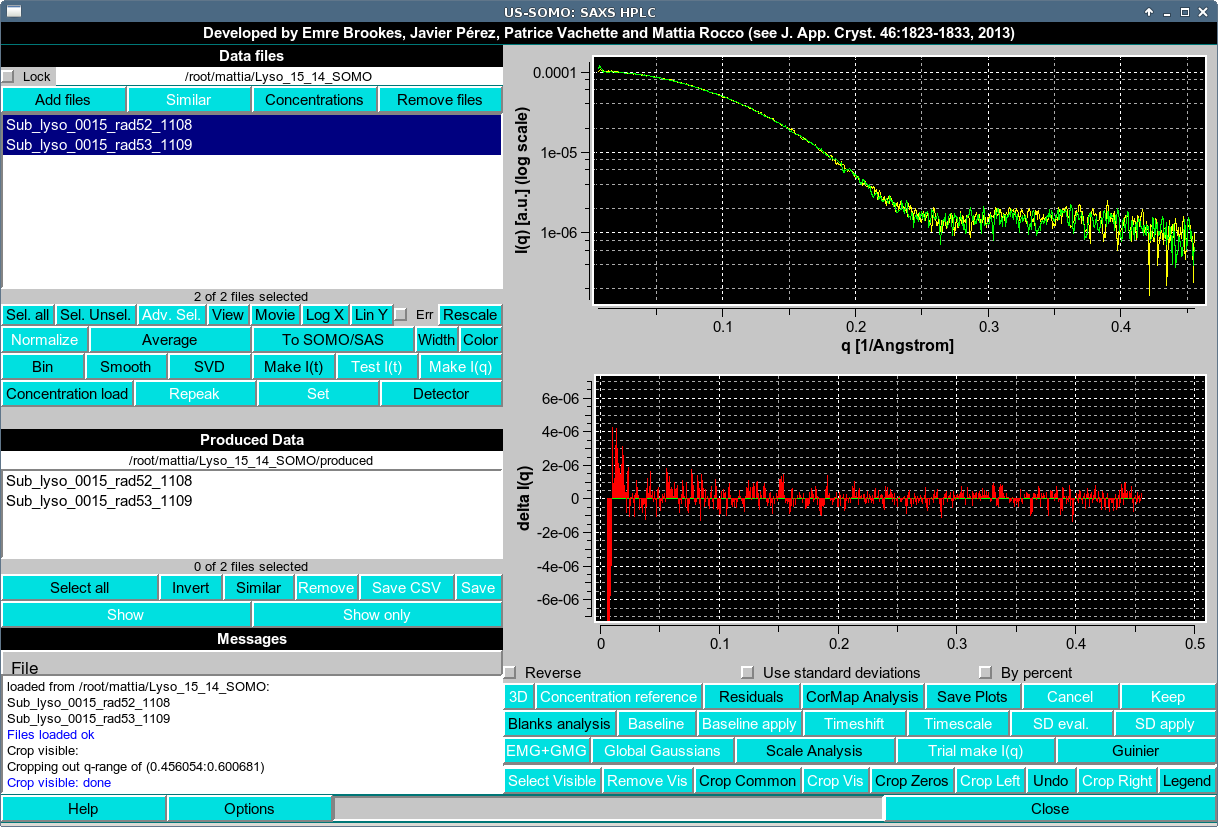
We wish to know if these two curves are P-value map probabilistically identical. This can be achieved by pressing the CorMap Analysis button in the first row under the plot. This will result in the following pop-up window:

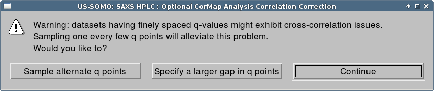
This window is asking if you wish to sample alternate q-points. Generally, the need for this depends on the beamline/detector characteristics, and is best evaluated during the analysis of Blanks (the frames typically averaged for buffer subtraction).

• Sample alternate q points will sample alternate q points.

• Specify a larger gap in q points will bring up another window (not shown) which will allow entry of an integer of value 3 or greater, to sample every specified number of q points.

• Continue will not sample and include all q points.

In this case will will press Continue to not sample. The following question:

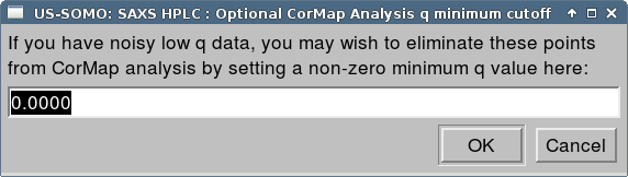
If you wish to remove noisy low q values from the CorMap analysis, you may enter a positive q value here. In our example, we press OK without changing the default value of zero. Finally, the CorMap Analysis window will be shown.

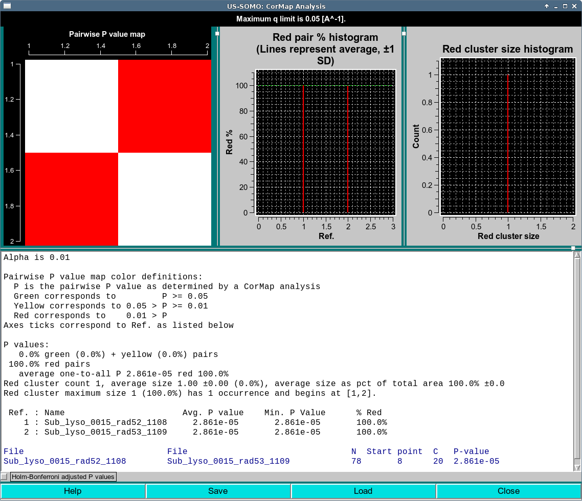
For clarity, we start with the bottom of the text area. In dark blue, the details of the CorMap comparison test(s) are listed. The two file names are first listed, then the number of q points compared N, followed by the q point position where the longest streak occurs (Start point), then the length of the longest streak (C) and finally the P-value of a streak of length C occurring in a sequence of N points.

In this case, we have long streak C of 20, starting at Start point 8. You can see this streak in the residuals plot shown in first image of this section.

The P values correspond to colors : green for P ≥ 0.05, yellow for 0.01 ≤ P < 0.05 and red for P < 0.01, as listed in the top of the text area.

In our example, this long C of 20 given an N of 78 points gives a P value < 0.01 and therefore encodes as red.

At the top left is the Pairwise P value map. This map summarizes the P value colors. The map is symmetric. The first row corresponds to the first file as summarized in the Ref. : Name section of the text area. The axis on the map are unfortunately not perfect, but the best we currently have (as in this case it unfortunately reports fractional values and the numbers are obviously not centered). In this trivial example, the map is a simple 2x2 since we are only comparing two I(q) data files. The diagonal is white, as it represents self-comparisons. The off-diagonal elements show the color of the P value comparison of the (i,j) curves.

At the top center is the Red pair % histogram. This histogram reports the percentage of red pairs in each row (or equivalently, column) as enumerated by Ref. of the map. There is a green horizontal line representing the overall average and also a yellow dotted lines at ± 1 S.D. (superimposed on the average in this trivial case, more informative examples are shown in the Scale mode and Baseline mode examples below).

At the top right is the Red cluster size histogram. A red cluster is defined as horizontally and/or vertically contiguous red points in the Pairwise P value map. In this case, we have simply a cluster size of one, and this is reported in the histogram. More complicated cases are reported the Scale Mode and Baseline Mode analyses below.

The text area contains in this order:

• The current Alpha level used for the analysis as defined in the Global CorMap Analysis alpha field of the HPLC SAXS Options.

• The color encoding information.

• Summary values for overall percentage of green plus yellow and red pairs.

• The overall average one-to-all average P value and red percentage of these pairwise comparisons.

• Statistics regarding the red clusters including the number of red clusters (red cluster count), their average size, and as a percent of total area.

• The Ref. to Name encoding, as well as the average and maximum P value for each entry compared to all other entries.

• In dark blue, the detailed comparison of each pair including their names, the number of points N, the Start point, the length of streak C and the P value

Below the text area is a checkbox labeled Holm-Bonferroni adjusted P values. Selecting this check box will replace the data with an Holm-Bonferroni adjusted version, which is not relevant in this trivial case of 2 curves. An example of Holm-Bonferroni adjusted data is shown here and here.

At the bottom of the window are four buttons

• Help will open documentation for this module in a web browser.

• Save will save the results in a csv file. This can be loaded in this module or in the Baseline utility of the main HPLC-SAXS window when in Integral Baseline mode of HPLC SAXS Options.

• Load will load a previously Saved csv file.

• Close will close the window.

Note the title within the window (not the window caption at the very top) lists specific information about the current CorMap analysis. These include:

• (...) mode will report the "mode" of the CorMap Analysis. This can have one of the following values:

  • Blanks mode is reported if CorMap Analysis was done with in the Blanks analysis as described the main HPLC-SAXS window documentation.

  • Baseline mode is reported if CorMap Analysis was performed from the Baseline utility of the main HPLC-SAXS window when in Integral Baseline mode of HPLC SAXS Options. This is also reported when the Find best region is selected within that utility, as it brings up a CorMap Analysis window automatically. Baseline mode will report the frame range in the title.

  • Scale mode is reported if CorMap Analysis was done with in the Scale analysis as described the main HPLC-SAXS window documentation. Scale mode will report the scaling range in the title.

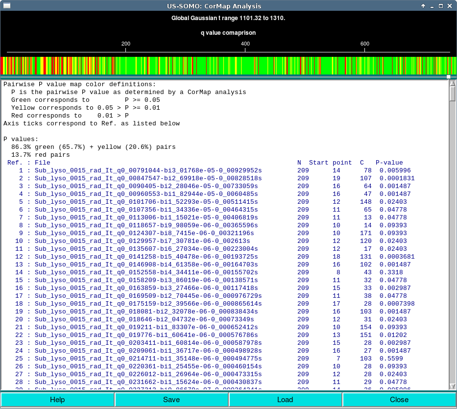
  • Global Gaussian mode is reported if CorMap Analysis was done with in the Scale analysis as described the main HPLC-SAXS window documentation. Global Gaussian mode will report the frame range in the title.

• Maximum q limit [A^-1] reports the maximum q value that is used for comparisons. This global value can be set in HPLC SAXS Options. A value of 0.05 is the default value to focus the comparison on the region of maximum signal intensity and also increase the sensitivity of the test.

• Minimum q limit [A^-1]. reports the minimum q value that is used for comparisons. This will only be displayed if an optional positive q value minimum limit has been specified for this CorMap analysis.

• Only every (...) q value sampled will be reported if sampling was used to generate the CorMap Analysis along with the sampling interval selected.

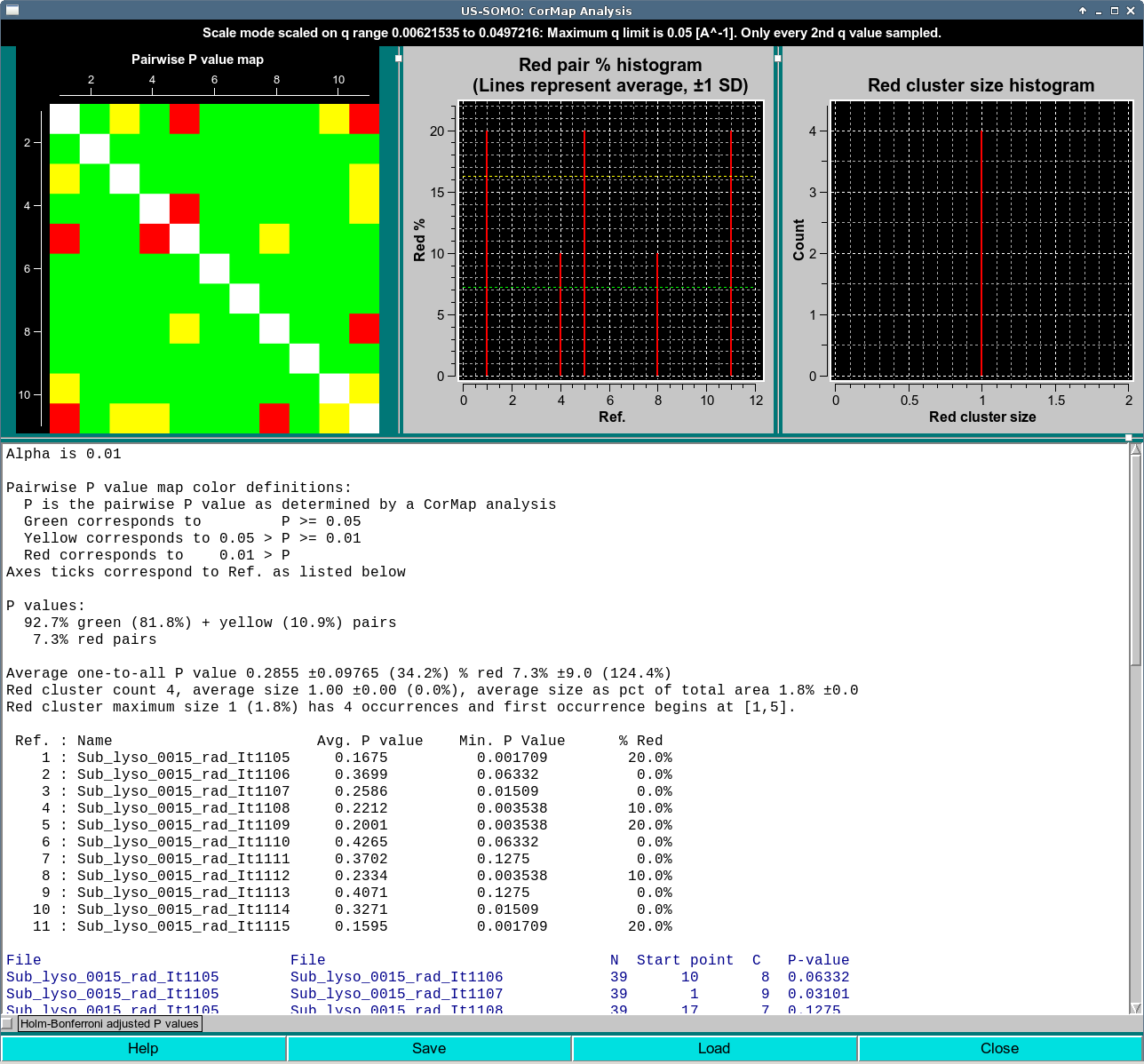
In this case, the CorMap analysis was performed on 13 curves from the top of a peak from the same Lysozyme data with alternate q point sampling. This is indicated in the window title with the text Only every 2nd q value sampled

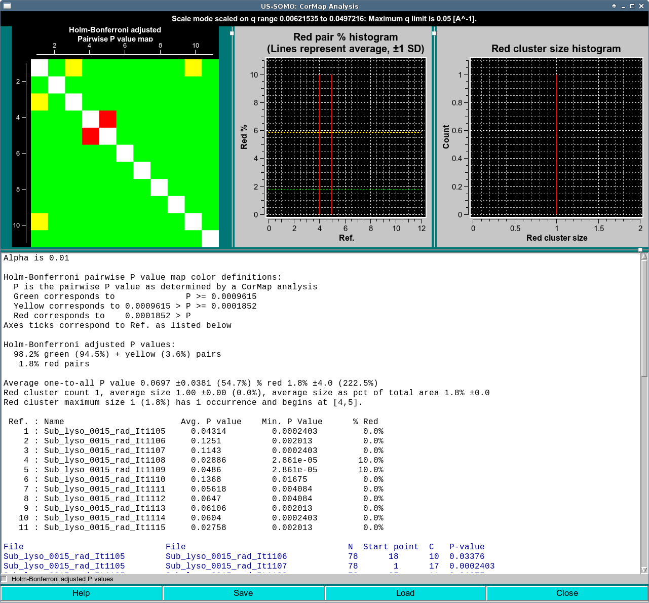
In this case, the CorMap analysis was performed on 13 curves from the top of a peak from the same Lysozyme data with with Holm-Bonferroni adjustment applied and without alternate q point sampling. Running the Holm-Bonferroni adjusted analysis with the alternative q value sampling as above results in a completely green map. Notice from the text area that the P-values limits have changed. These are the values as determined after application of the Holm-Bonferroni adjustment.

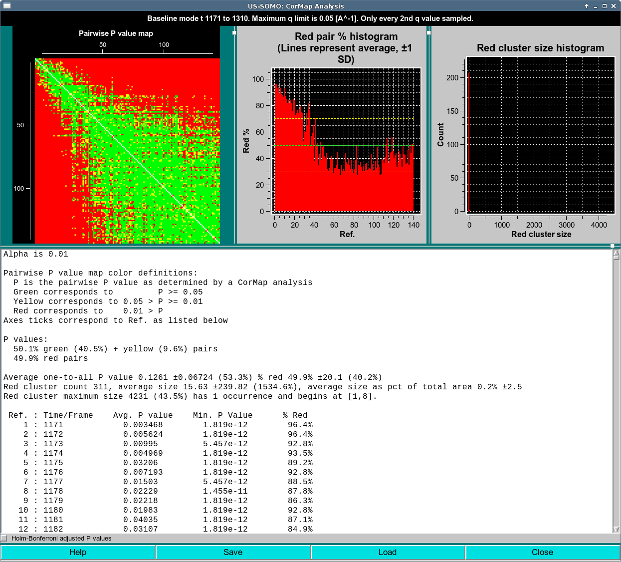
In this case, the title also reports the frame range. The range selected includes the eluting peak, so a lot of red occurs as I(q)'s change. A stable region is observable in the lower right as large, predominantly green diagonal sub-blocks appear.

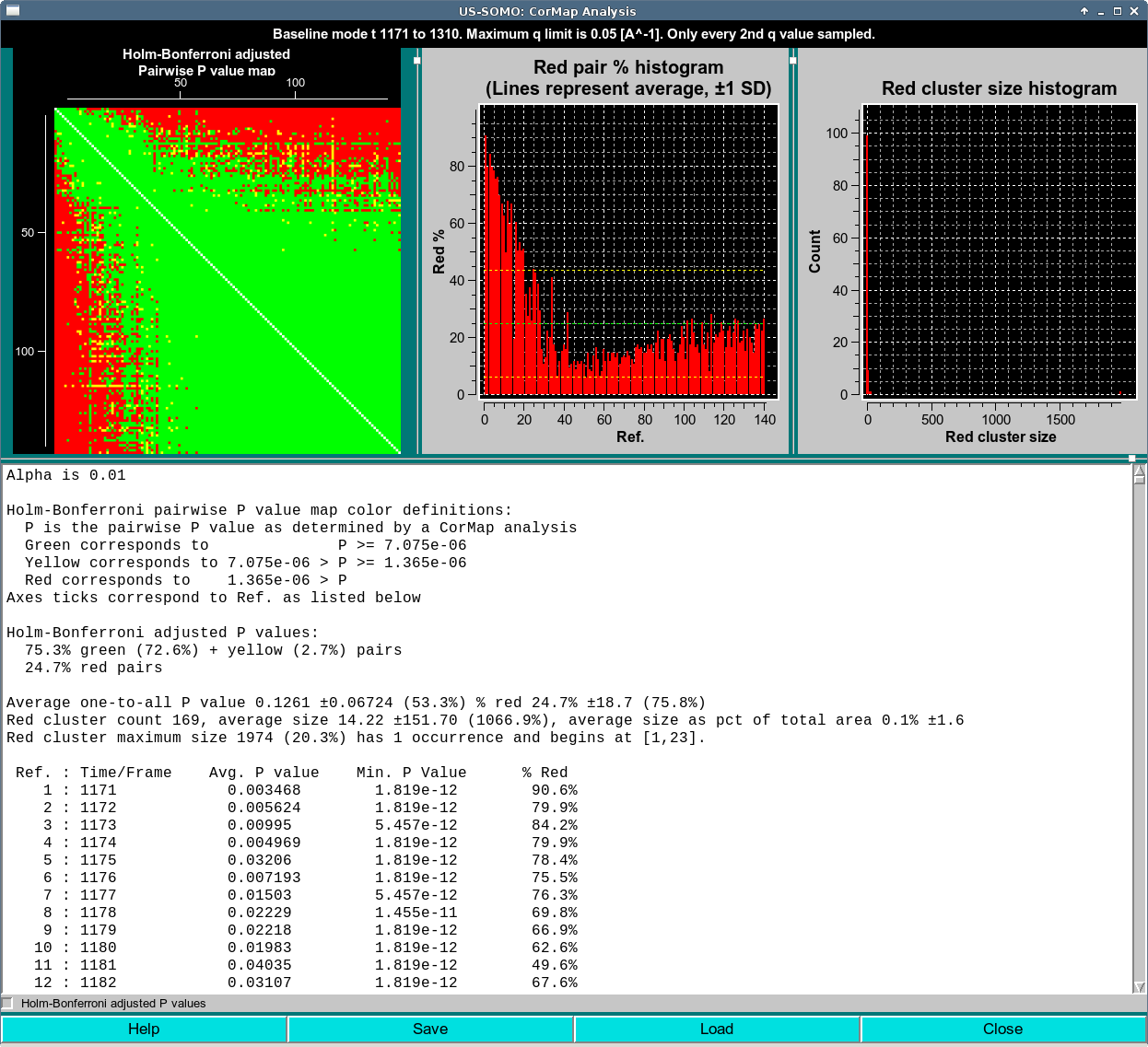
This is the idential dataset to the previous analysis with the same sampling. The only difference is the Holm-Bonferroni adjustment was applied. As above, the range selected includes the eluting peak, so a lot of red occurs as I(q)'s change. A large stable region is observable in the lower right as a completely green diagonal sub-block. As with the Scale mode analysis with Holm-Bonferroni adjustment, notice from the text area that the P-values limits have changed. These are the values as determined after application of the Holm-Bonferroni adjustment.

In this case, the CorMap analysis is different from the standard CorMap analysis, and the button to access it changes from CorMap Analysis to Show CorMap to reflect this difference. The CorMap comparison is done between I(t) curves and their Gaussian representation, resulting in a single row of colors in the map, one for each I(t) and is Gaussian representation. There is also no red cluster information, as this is only applicable to a two dimensional map. (This mode does not currently support Load.)

This document is part of the UltraScan Software Documentation distribution.
Copyright © notice.

The latest version of this document can always be found at:

http://somo.aucsolutions.com

Last modified on December 13, 2017.