Manual

Last updated: December 2017

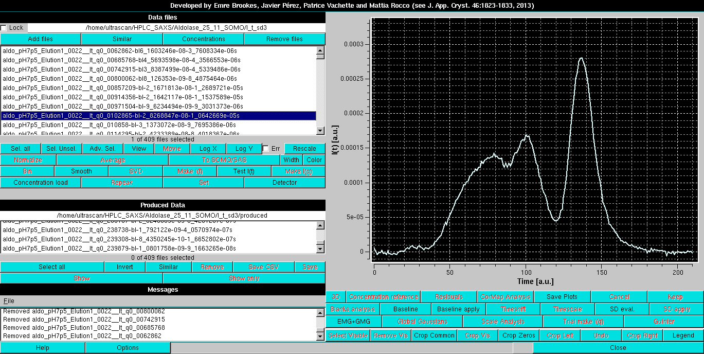
This manual part describes the Gaussian analysis and decomposition operations using non symmetrical (skewed, distorted) Gaussians. The dataset we will use as an example is the same HPLC-SAXS analysis of Aldolase that is used to demonstrate the linear baseline operations (see here):

The type of distorted Gaussian to be utilized is chosen in the Options panel accessed by pressing the Options button:

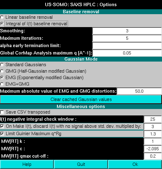
We will start with the Exponentially modified Gaussian (EMG) function. After selecting it and returning to the HPLC-SAXS main panel, a EMG button will replace the default Gaussians button. Pressing it will bring up the EMG settings:

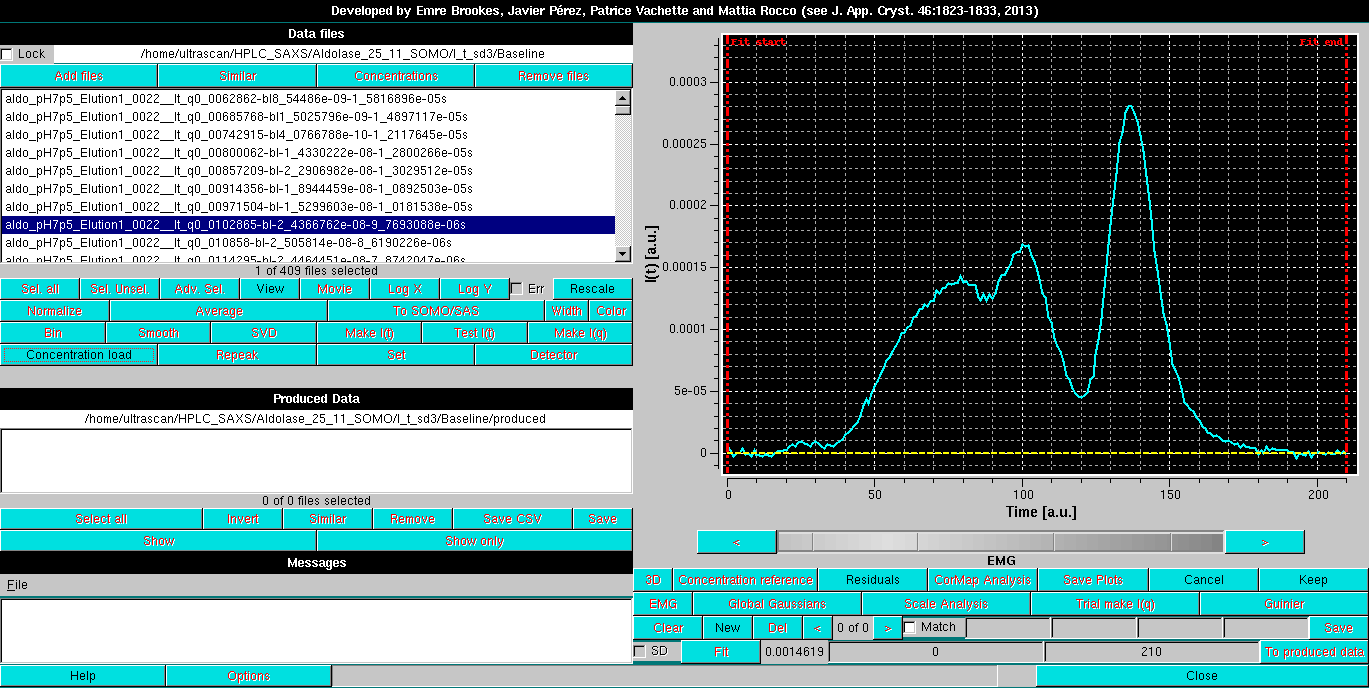
Since an SVD analysis (see here) on this dataset (not shown) indicated that four components were at least needed to describe it, four EMG Gaussians are initally positioned:

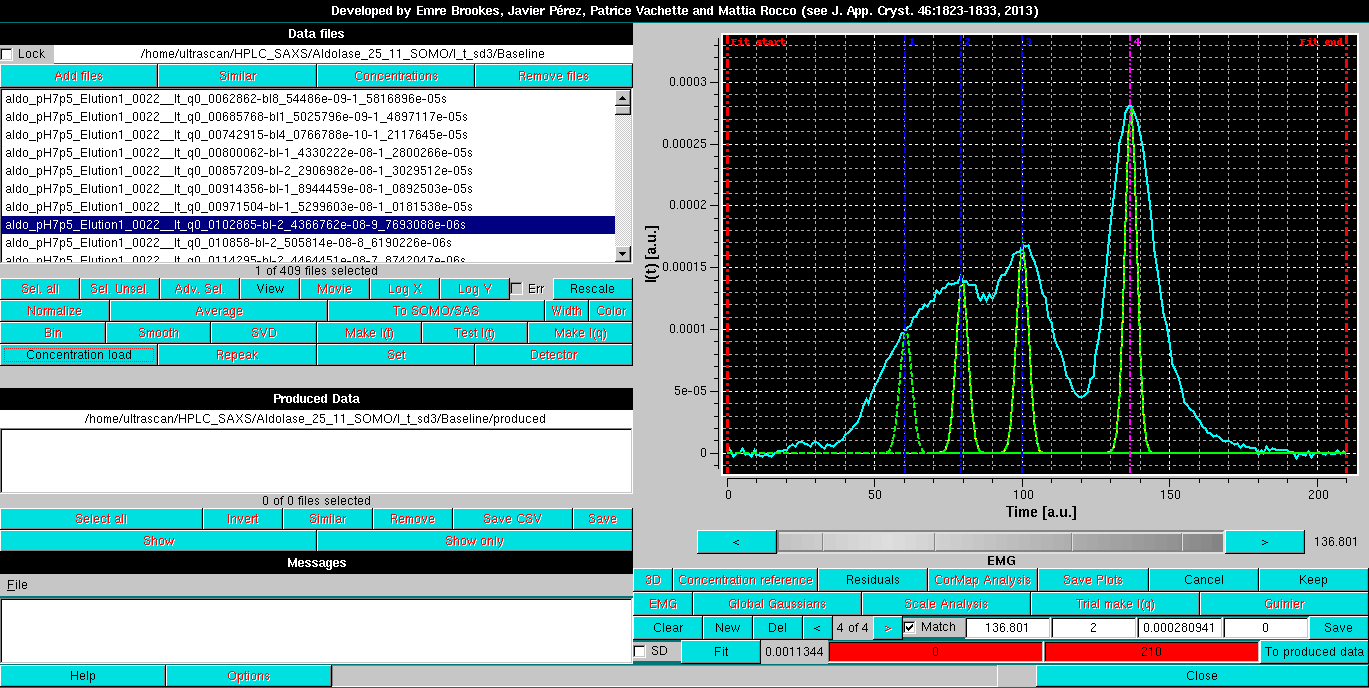
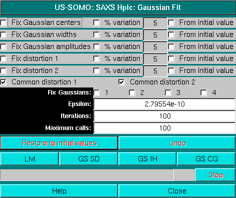
Note that four fields are now present in the third commands row. The first three are the center, width and amplitude of each Gaussian, as in normal Gaussian operation, while the fourth is the EMG Gaussian distorsion (set to 0 at the beginning). All other commands are identical as for normal Gaussian operations. Once the intial set of EMG Gaussians is positioned, pressing Fit will bring up again the Gaussian Fit module:

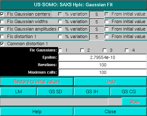
Note that in respect to the normal Gaussians operation, there is an additional distorsion field with its checkboxes (Fix distortion 1, % variation, and From initial value), and a Common distorsion 1 checkbox. The latter is selected by default, because it is assumed that similar species will have similar distorsions on eluting from the column. This makes the Gaussian fitting more robust. If necessary, once an initial round of fitting is performed, this constraint can be released, to verify if any further improvements are possible while still keeping resonable peak shapes for all Gaussians.

As with normal Gaussain operation, it is advisable to do a first fit while keeping the Fix Gaussian centers checkbox selected:

Followed by a round with the centers restrained by the % variation 5 from initial value:

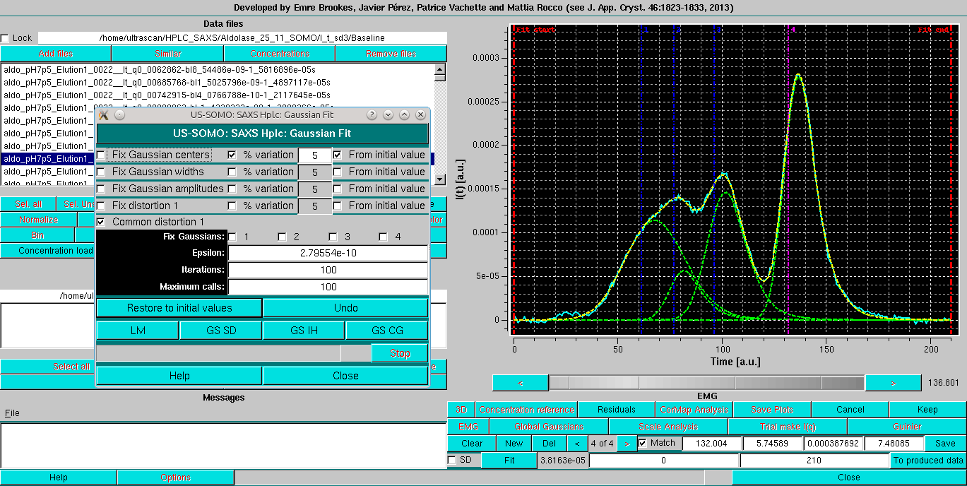
Bringing in the SD and releasing all constraints but the Common distorsion produces a slightly improved fit:

However, the cost paid to achieve this apparently quite satisfactory fit is that the contribution of peak #1 appears to be exaggerated.

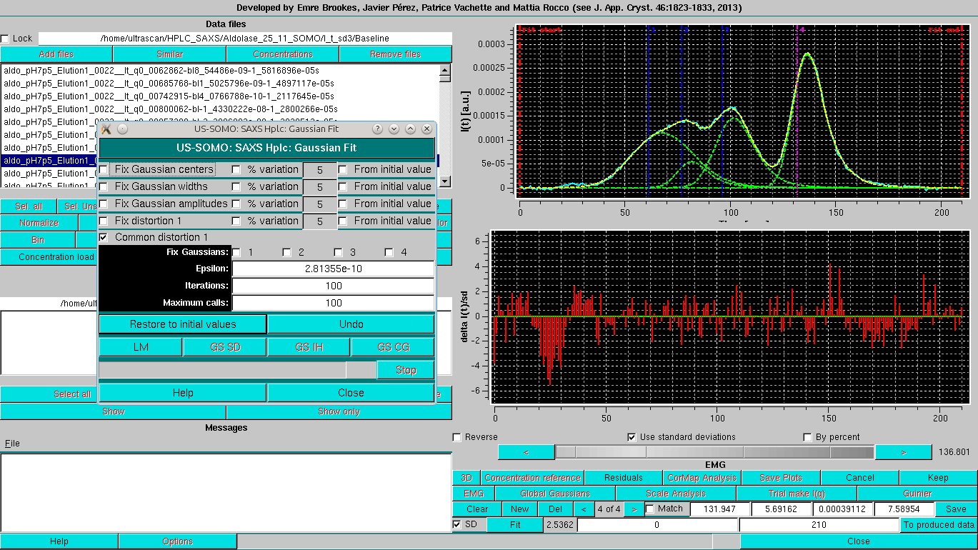
We can perform the same analysis using the Half-Gaussian modified Gaussian function:

As can be seen from the fit χ² (next to the Fit button), this function performs worse for this dataset. A function combining the EMG and GMG Gaussians (EMG+GMG) can be also tested. The corresponding Fit module will present extra fields:

see here for a complete description description of the Fit module. In addition, we will also restrict the fitting region, to help improve the fitting. The results of this EMG+GMG fitting are shown below:

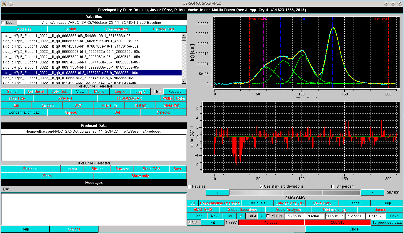
As can be seen, there is a substantial improvement, mainly due to the exclusion of the small bump before the first peak. We will then proceed with this set, first by doing Global Gaussians on a subset:

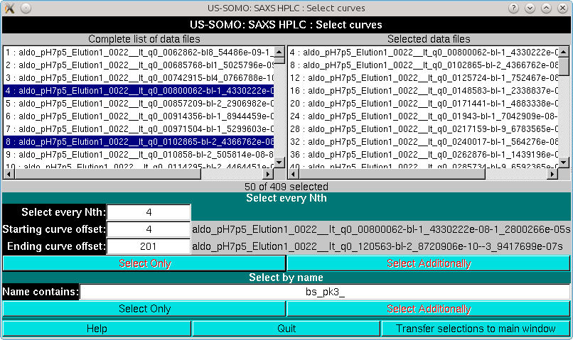
and then proceeding with Global fit:

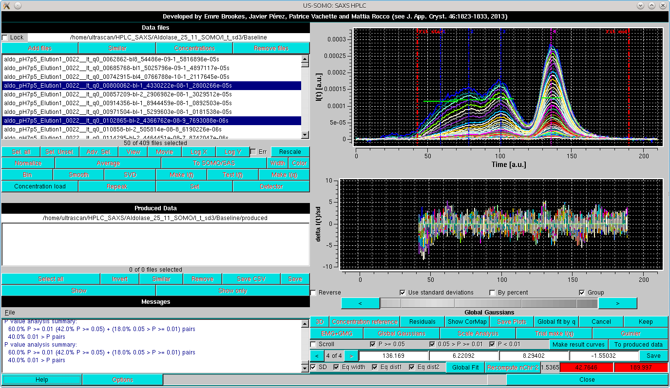
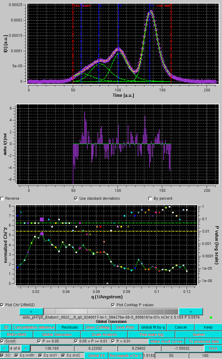
Here, already by looking at the Residuals, the fit appears to be improved, and the apparently larger residuals especially around the main peak are due to the very low SD associated with the data, amplifying the discrepancies. The goodness of the fit can be further checked by first resticting again the fit limits, then recomputing the residuals by pressing Recompute nChi^2, and subsequentely pressing Global fit by q:

This will bring up an additional plot where the normalized χ² (diamonds connected by a line) and the pairwise CorMap P-values (squares) are plotted as a function of the q-value. In the Global fit by q graph it is possible to visualize either one of or both the two plots, by selecting/deselecting their respective checkboxes positioned just below it (Plot Chi^2/RMSD and Plot CorMap P values). Note that in the image above, where both plots are shown, their respective y-axis scales have been manually modified to allow a better visualization of each plot. The dashed green and yellow horizontal lines mark the usual cut-off P-values (P ≥ 0.05, above the green line; 0.05 > P > 0.01 between the green and yellow lines; P < 0.01, below the yellow line).

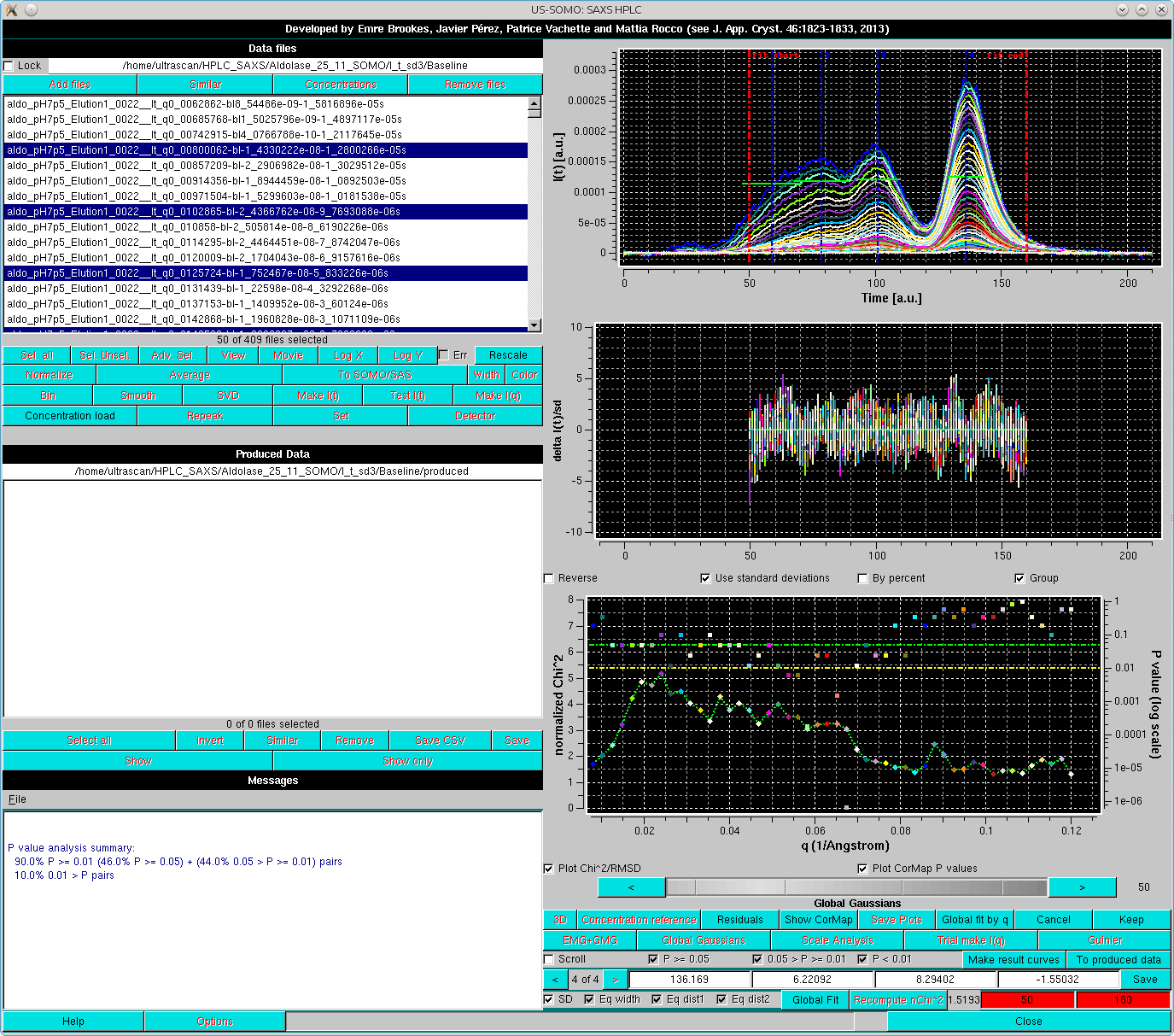
The correlation between the goodness-of-fit indicators and the distribution of the residuals can be examined for each original/fit I(t vs. t pair by selecting the Scroll checkbox:

The current chromatograms pair is highlighted in both plots by an enlarged symbol (purple square in this case). Scrolling is performed by either using the grey-scale bar-wheel, or by clicking on the the "<" and ">" buttons placed at its sides. By selecting/deselecting the three checkboxes next to the Scroll checkbox (P >= 0.05, 0.05 > P >= 0.01, P < 0.01), only the subset(s) whose P-values are within those of the selected chechbox(es) will by scrolled.
Note how here to a relatively "bad" χ² value (5.169) corresponds a "good" CorMap value (P = 0.0974). This indicates an essentially random residual distribution, while the high χ² value is mainly due to the very low SD associated with the data, since the fit appears also to be quite good (top graph).

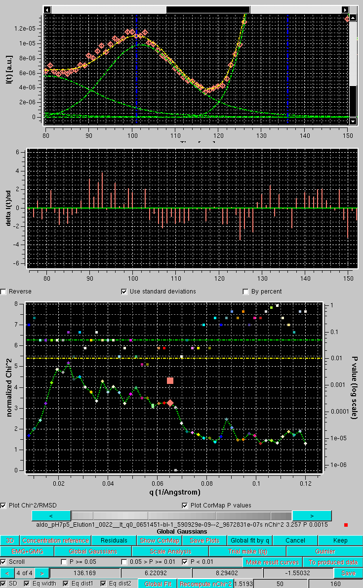
Conversely, if we examine a q-value where the χ² is better (3.257) but the P-value is bad (0.0015), we can see by zooming on the inflexition between the 3^rd and 4^th peaks that the latter is mainly due to a stretch of I(t) experimental values (salmon diamonds) sligthly below the EMG+GMG fit curve:

After accepting the Global Fit, the EMG+GMG Gaussians are then propagated to all chromatogram by first selecting all chromatograms amd then pressing Global Gaussians:

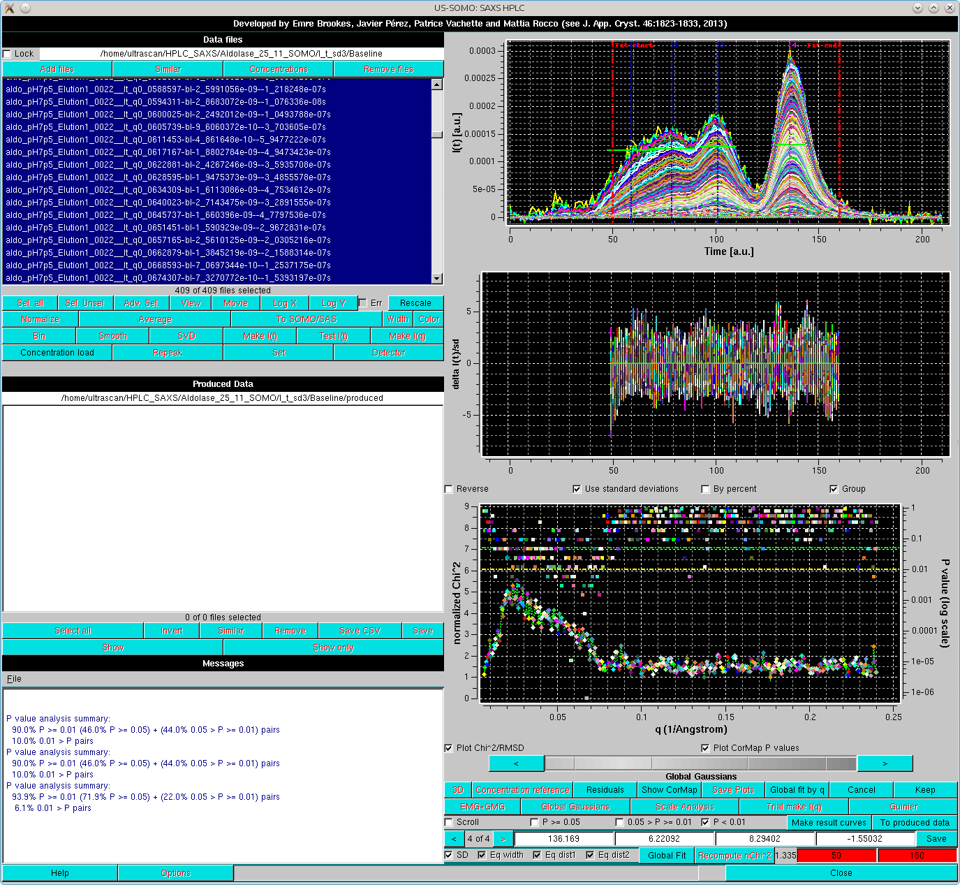
where the goodness of the reconstruction can be appreciated in both the Reduced Residuals and the Global fit by q plots.

Save and Keep can then be sequentially pressed to store and accept the global Gaussian results. After non-symmetrical Gaussian decomposition, the Trial make I(q) procedure can be launched to further test the results, as described in the main Help pages.

This document is part of the UltraScan Software Documentation distribution.
Copyright © notice.

The latest version of this document can always be found at:

http://somo.aucsolutions.com

Last modified on December 13, 2017.